Strategic Communication with Lying Costs
Abstract.
I study a model of strategic communication between an informed Sender and an uninformed Receiver. The Sender bears a cost of lying, or more broadly, of misrepresenting his private information. The main results show that inflated language naturally arises in this environment, where the Sender (almost) always claims to be a higher type than he would under complete information. Regardless of the intensity of lying cost, there is incomplete separation, with some pooling on the highest messages. The degree of language inflation and how much information is revealed depends upon the intensity of lying cost. The analysis delivers a framework to span a class of cheap talk and verifiable disclosure games, unifying the polar predictions they make under large conflicts of interest. I apply the model to highlight how the degree of manipulability of information can affect the tradeoff between delegation and communication.
Key words and phrases:
Cheap Talk, Signaling, Misreporting, Exaggeration, Disclosure, Persuasion, Delegation.1. Introduction
The strategic transmission of private information plays an important role in many areas of economics and political science. Most theoretical studies of direct communication can be classified into the following two categories. One approach, initiated by Grossman (1981) and Milgrom (1981), assumes that information is verifiable and agents can withhold information but not lie. These are referred to as games of “persuasion” or “verifiable disclosure.” The second approach, pioneered by Crawford and Sobel (1982) and Green and Stokey (2007, circulated in 1981), assumes that information is unverifiable and an agent can lie arbitrarily without direct costs, typically referred to as games of “cheap talk.”
These are two extremes in a continuum of possibilities. Rather than lying — synonymous in this paper with misrepresentation or misreporting — being completely costless or prohibitively costly, reality usually lies in between: individuals can and do misrepresent private information, but bear some cost in doing so. These costs arise for various reasons. First, there may be probabilistic ex-post state verification that results in penalties if misreporting is detected, such as random audits on taxpayers (e.g. Allingham and Sandmo, 1972). Second, there may be costs of manipulating information or falsifying a message, such as when a manager has to spend time “cooking the numbers” or otherwise expend costly resources in order to report higher profits (e.g. Lacker and Weinberg, 1989; Maggi and Rodriguez-Clare, 1995). Third, recent experimental work suggests that people have an intrinsic aversion to lying, even though messages are prima facie cheap talk (Gneezy, 2005; Hurkens and Kartik, 2008; Sánchez-Pagés and Vorsatz, 2006).
This paper studies the classic strategic communication setting of Crawford and Sobel (1982) (hereafter CS), with the innovation that some messages entail exogenous or direct lying costs for the Sender. I use the term “lying costs” to broadly capture a class of misrepresentation costs, such as those discussed above. To fix ideas, here is a simplified version of the model presented in Section 2: a Sender is privately informed about his type, , and must send a message to the Receiver, who then takes a decision which affects both players’ payoffs. There is a conflict of interest because the Sender wants the Receiver to believe that his type is higher than it actually is. I suppose that for each Sender type, , there is a set of messages, , with the interpretation that any message has the literal or exogenous meaning “my type is .” In this framework, the Sender is said to be lying when he sends a message for some , and the magnitude of a lie can be measured by the distance between his true type and the type he claims to be. When type sends a message , he bears a cost , where is a scalar that parameterizes the intensity of lying cost. If , messages are cheap talk, and the setting reduces to that of CS. This paper is concerned with . Assume that for any , it is cheapest to tell the truth, and moreover, the marginal cost of a bigger lie is increasing in the magnitude of the lie.
Lying costs transform the CS cheap-talk model into one of costly signaling, although the induced structure is different from traditional “monotonic” signaling games (Cho and Sobel, 1990). The main results I provide concern the amount of information revealed by the Sender in equilibrium, and the language — the equilibrium mapping from types to messages — through which information is transmitted. For most of the paper, I focus on a tractable and appealing class of Perfect Bayesian equilibria, described in Section 3.111Although the possibility of other equilibria is not ruled out, these are the only ones that satisfy a refinement criterion proposed by Bernheim and Severinov (2003). The structure of these equilibria is simple: low Sender types separate, revealing themselves through their equilibrium message, whereas high types segment into one or more connected pools. The equilibria feature language inflation in the sense that (almost) every type sends a message for some . That is, the Sender (almost) always claims to be a higher type than he truly is, even though he suffers a cost of lying. Of course, the Receiver is not systematically deceived, because she recognizes that the Sender is inflating his messages and adjusts her decision accordingly. While this state of affairs may appear paradoxical at first glance, the key point is that if the Sender were to tell the truth (i.e. send a message when his type is ), the Receiver would infer that his type is in fact lower than it actually is, since she expects messages to be inflated. There is thus an inescapable inefficiency for the Sender in equilibrium, reminiscent of unproductive education signaling in Spence (1973) or dissipative advertising in Milgrom and Roberts (1986a).
Language inflation is difficult to explain in a framework of pure cheap talk, due to the indeterminacy of language in any cheap-talk game. Yet, the phenomenon occurs in numerous settings of communication with conflicts of interest. For example, analysts at brokerage firms that have an underwriting relationship with a stock tend to provide inflated recommendations on that recommendation (e.g. Lin and McNichols, 1998; Michaely and Womack, 1999). The literature discusses two basic forces that determine an affiliated analyst’s incentives: first, the existence of an underwriting relationship creates a pressure to induce clients to buy the stock; second, there are present compensation and future reputation rewards for more accurate recommendations. In terms of my model, the more an analyst’s compensation is determined by accurate assessments, the higher is the intensity of lying costs, .222Of course, there may be an additional component to lying costs stemming from regulatory concerns. I establish some intuitive and testable comparative statics with respect to this intensity. At the extreme case, as , equilibria converge to full separation with almost no language inflation, i.e. there is close to truth-telling. On the other hand, as , there is a lot of pooling with extremely inflated language.
In Section 4, I analyze in detail a canonical parametrization of the model, based on CS’s influential “uniform-quadratic” example. This permits closed form solutions for equilibria in a wide range of lying costs, and delivers additional comparative statics to those mentioned above. I then briefly apply these results to revisit the question of optimal allocation of authority in organizations between an informed agent and uninformed decision-maker. Dessein (2002) showed that a decision-maker prefers cheap-talk communication to unconstrained delegation if and only if the conflict of interest is sufficiently large. In contrast, I find that whenever the lying cost intensity is not too small in the leading example, communication can dominate delegation regardless of the conflict of interest. More generally, my results indicate that the tradeoff between communication and delegation will depend upon how costly it is for the agent to manipulate information.
Section 5 proposes an extension to span the cheap talk and verifiable disclosure approaches to strategic communication. As previously noted, the verifiable disclosure literature assumes that the Sender cannot lie about his type, but can withhold information. Not being able to lie may be viewed as the limit of my model as . To capture the ability to withhold information, I augment the model so that the Sender can make vague statements about his type, including being silent altogether at no cost. The main results are extended to this setting. One consequence is that when the conflict of interest between Sender and Receiver is large, the current framework unifies the dichotomous results of unraveling (full information revelation) in verifiable disclosure games and babbling (no information revelation) in cheap-talk games.
To summarize: the analysis here shows how lying costs can significantly affect the outcome of strategic information transmission. Consequently, direct communication may have a greater scope to reduce the costs of asymmetric-information-based incentive problems than otherwise suggested. This theoretical finding is consistent with experimental evidence, where “overcommunication” is often documented (e.g. Cai and Wang, 2006). Section 6 concludes with some comments on economic implications and potential applications of the current framework.
1.1. Related Literature
This paper contributes to the literatures on cheap talk, costly signaling, and verifiable disclosure. Most closely related to my work are the following contemporaneous papers: Chen (2007), Chen et al. (2008), Kartik et al. (2007), and Ottaviani and Squintani (2006). I now discuss the connections in some detail, followed by a briefer mention of other related work.
Kartik et al. (2007) also study the notion of costly lying and language inflation. However, the focus and analysis is quite different, because they study an unbounded type space setting. They prove the existence of separating or fully-revealing equilibria for arbitrarily small intensity of lying cost (and other costly signaling structures).333Austen-Smith and Banks (2000) analyze a model of cheap talk and costly signaling, where the costly signal takes the form of “burned money.” That is, the cost of the signaling instrument does not vary with the Sender’s type. Their focus is on how the presence of this additional instrument can enlarge the set of CS equilibria, with a key result that so long as the Sender’s ability to impose costs on himself is sufficiently large, separating equilibria exist. Kartik (2007) shows that as the ability to burn money shrinks to , the set of equilibria in Austen-Smith and Banks (2000) converges to the entire set of CS equilibria. Kartik (2005) discusses the differences between burned money and costly lying. This result relies essentially on the unboundedness of the type space, because the Sender is then able to inflate his message without restraint. In contrast, in this paper I study the canonical bounded type space model of CS, and show that separating equilibria do not exist regardless of the lying cost intensity.444This statement requires some caveats when the setting is more general than that described in this introduction; see Theorem 1 and fn. 10. Intuitively, given that messages must be inflated, the upper bound on the type space acts as a barrier to full separation. Consequently, the attention here is necessarily on partially-pooling equilibria. Aside from requiring a more complex analysis, this also permits me to address issues that cannot be meaningfully answered in an unbounded type space model, such as large conflicts of interest and comparative statics of partial-separation.
In a bounded type space, Ottaviani and Squintani (2006) study the “uniform-quadratic” specification of CS. They introduce the possibility that the Receiver may be naive or non-strategic. This transforms the game from one of cheap talk into a costly signaling structure that can be subsumed by the current framework (see Section 2.1). For some parameterizations, they construct an equilibrium that has similar features to the equilibria studied here. Their parametric restrictions require the conflict of interest between Sender and Receiver to be sufficiently large relative to other parameters, which is not required here. Ottaviani and Squintani (2006) provide some comparative statics that are complementary to those in this paper. There is no analog in their work to the analysis I undertake in Section 5 about withholding information.
Chen (2007) furthers the non-strategic approach by modeling not only Receiver naivety, but also Sender naivety or mechanical honesty. Specifically, she posits that with some probability the Sender just reports his type truthfully, and with some independent probability the Receiver takes the message to be truthful. Using the uniform-quadratic specification of CS, she shows that there is a unique equilibrium in the cheap-talk extension (Manelli, 1996) of her model that satisfies a monotonicity requirement. Language is inflated in her equilibrium, for reasons similar to this paper, since Receiver naivety induces a particular form of lying costs. A benefit of assuming Sender naivety is that it ensures that all messages are used in equilibrium, obviating the need to consider off-the-equilibrium-path beliefs.555The specification of Sender naivety imposes particular restrictions on beliefs when a message is observed that is not sent by a strategic Sender. In effect, it substitutes for restrictions on off-the-equilibrium-path beliefs in a fully rational model. A strength of the approach here is that both the underlying cheap-talk model and the costly signaling structure are more general.
Chen et al. (2008) propose a refinement called No Incentive to Separate (NITS) for cheap-talk games like CS. Among other justifications for the criterion, they show that only CS equilibria satisfying NITS can be the limit of certain equilibria in a class of games with lying costs, as the intensity of lying costs shrink to . Although their model does not strictly subsume the current setting, their arguments can be adapted. The analysis here is entirely complementary, because I study arbitrary intensities of lying cost, rather than just the cheap-talk limit as the costs vanish. Inter alia, this paper provides an explicit characterization of a set of equilibria for any cost intensity.
With regards to the broader signaling literature, I build upon techniques developed by Mailath (1987) to study costly signaling with a continuum of types. Whereas his analysis concerns separating equilibria, the main results in this paper concern partially-pooling equilibria, as already noted. Cho and Sobel (1990) were the first to derive incomplete separation in the manner obtained here: pooling at the top of the type space using the highest messages and separation at the bottom. Their analysis is for a class of signaling games that have a finite type space and satisfy a single-crossing property that does not apply to the current setting. A more closely related model is that of Bernheim and Severinov (2003). Although they study a topic in public finance and the issues we each focus on are rather different, the formal structures have similarities. My equilibrium characterization builds upon their work.
Lastly, I should also briefly mention two other literatures that touch upon related issues. First, there is a small literature on contracting and mechanism design with misrepresentation costs, initiated by Green and Laffont (1986). Generally, the costs are taken to be either zero or infinite, but see Deneckere and Severinov (2007) for an exception. Second, there are some papers in accounting that propose signaling theories of earnings management, e.g. Stein (1989). They also motivate costly misreporting for technological or legal reasons, but to my knowledge only consider unbounded type spaces and special functional forms.
2. The Model
There are two players, a Sender () and a Receiver (). The Sender has private information summarized by his type , which is drawn from a differentiable probability distribution , with strictly positive density for all . After privately observing his type , the Sender sends the Receiver a message, , where is a Borel space of available messages. After observing the message, takes an action, .
I assume that , with for all and if . The interpretation is that any carries the literal or exogenous meaning “my type is .” Since is a partition of , any can be associated with a unique such that ; denote this mapping by . Thus, if , the Sender is claiming in literal terms to be a higher type when he sends rather than , and I will say that is higher or larger than (only weakly, if ).
The payoff for is given by , and the payoff for is given by . Here, and represent the two players’ preferences over type-action pairs, whereas is a lying cost function, is a scalar that parameterizes its intensity, and is a function that will be further discussed below. Note that is payoff-relevant only for . All aspects of the game except the value of are common knowledge.
I now introduce two sets of assumptions on players’ preferences. The first set is identical to Crawford and Sobel (1982), while the latter defines the costs of lying.
Preferences over actions: For , the function is twice continuously differentiable on .666More precisely, there exists an open set containing and two twice continuously differentiable functions on which are respectively identical to and on . Analogous statements apply to subsequent assumptions about differentiability of and . Using subscripts to denote derivatives as usual, for , so that both players’ payoffs are concave in ’s action and supermodular in . For any , there exists and respectively such that , with . That is, the most-preferred actions are well-defined for both players, and the Sender prefers higher actions than the Receiver. These assumptions imply that for , , i.e. both players prefer higher actions when the Sender’s type is higher.
Preferences over messages: The function is continuously differentiable on and strictly increasing. The function is twice continuously differentiable on , with . These assumptions imply that there is a continuous and weakly increasing function, , such that for any , . In words, is the type that would claim to be in order to minimize message costs. Equivalently, any is a cost-minimizing message for . I assume that , but nothing else about the function . The assumptions on and imply that when is farther from , is more costly for , and moreover, the marginal change in cost from claiming to be a slightly higher type than is larger in absolute value.
2.1. Discussion.
Here are some comments on the model’s assumptions and interpretations.
Message space.
As mentioned, each message is associated with some type, with the interpretation that every statement the Sender can make has a literal meaning about the exact value of his type.777Section 5 shows how the model can be extended to cases where the Sender is permitted to make “vague” statements about his type (e.g., “my type lies in ”). An alternative interpretation is that the Sender must submit some evidence or data to the Receiver, and his type represents the true realization of this evidence, which is costly to falsify. The assumption that each contains an infinite number of messages may be viewed as assuming a rich language: there are a large number of ways in which the Sender can make a statement with the literal content that his type is , for example, “my type is ,” or “you should believe that my type is ,” and so forth.888An infinite number of messages in each is a stronger assumption than necessary; a large enough finite number would always do. Some of the results only require . It is worth noting that a special case of the model is when the Sender can make a two-dimensional statement about his type: on one dimension he reports an exact value about his type and suffers a cost of misreporting the truth, while on the other, he just makes a cheap-talk statement from some arbitrary (infinite) set. For example, firms can take costly actions to manipulate earnings reports that must be submitted, but they can also simultaneously provide costless explanations or justifications.
Lying costs.
If , the model reduces to the cheap-talk model of CS. Since , messages are discriminatory signals in the sense that the cost of a message varies with the Sender’s type. An important example to keep in mind throughout the analysis is as follows: , and for all (e.g., ). In this case, , i.e. it is cheapest to tell the literal truth.
The assumption means that the highest type minimizes cost by claiming to be itself. Obviously, this assumption is satisfied when it is cheapest for each type to tell the truth. It also holds in an application discussed below, even though truth-telling is not cost-minimizing for all types there. In any case, the assumption is made primarily for expositional convenience; all the analysis can be generalized to settings where , as pointed out in fn. 10.
Let me emphasize that the Sender’s costs of lying in this model depend only upon his type and the message he uses. Plainly, this is appropriate when the costs stem from potential auditing penalties or technological/opportunity costs of falsifying information. In terms of capturing psychological aversion to lying, the interpretation is that the Sender is averse to making statements that would be considered untruthful under a literal or otherwise exogenous interpretation of statements.999One might suggest that psychological costs of lying should take into account the Receiver’s endogenous interpretation of a message. While this is interesting, I leave it for future research. The assumption that costs are convex in the type that the Sender claims to be (holding fixed his true type) is a substantive but natural one. For example, it would arise if there is a fixed probability of misreporting being detected and penalties are convex in the magnitude of misreporting.
Naive Receivers.
Admitting the possibility that the Receiver may be naive or credulous can induce costs on the Sender that are similar to exogenous lying costs. To illustrate, suppose as in Chen (2007) or Ottaviani and Squintani (2006) that messages are cheap talk, but with probability , the Receiver is (perceived to be) credulous, in which case she takes message at face value, responding with action . Now, when the Sender is of type , the expected utility from sending message and receiving action from a strategic Receiver is given by
Setting , , and , the above payoff expression can be normalized and rewritten as . The properties of and imply that and thus defined satisfy my assumptions. Note that in this case,
and is therefore not strictly increasing. Indeed, if the conflict of interest between Sender and Receiver is sufficiently large (), is a constant function. Nevertheless, is weakly increasing and satisfies .
2.2. Strategies and Equilibrium.
A pure strategy for the Sender strategy is a (measurable) function , so that is the message sent by type . Denote the posterior beliefs of the Receiver given a message by the cumulative distribution . A pure strategy for the Receiver is a function , so that is the action taken when message is observed. The solution concept is Perfect Bayesian Equilibrium (PBE), which requires the Sender to maximize utility for each type given the Receiver’s strategy, the Receiver to maximize utility given his beliefs after every message, and beliefs to satisfy Bayes’ rule wherever it is well-defined.
For most of the analysis, I only consider pure strategy PBE, which are referred to as just “equilibria” hereafter. Moreover, I typically restrict attention to equilibria where the Sender’s strategy is weakly increasing, in the sense that if , then . This property is called message monotonicity, and an equilibrium which satisfies the property is a monotone equilibrium. In a monotone equilibrium, the Sender makes a weakly higher claim about his type when his type is truly higher. Attention to such equilibria seems reasonable because higher types intrinsically prefer higher messages due to the cost of lying structure (formally, is weakly increasing).
3. Signaling and Inflated Language
3.1. Impossibility of Full Separation.
The basic signaling problem is that the Sender wants the Receiver to infer that he is a higher type than he actually is. Say that a type is separating if , i.e. the message sent by reveals that the Sender’s type is . A separating equilibrium is one where all types are separating. Naturally, the first question is whether such equilibria exist.
It is generally more convenient to work with the mapping directly, rather than just . Note that , and is interpreted as the type that claims to be.
Definition 1.
A type is said to be using inflated language if . A type is telling the truth if .
The above definition is appropriate because it compares what a type claims to be in equilibrium relative to what it would claim under complete information, i.e. if the Receiver knew the Sender’s type, which is by definition. Thus, truth-telling refers to what a type would say under complete information; whether it satisfies depends on the properties of and . Since under complete information the Sender would play a strategy such that , any deviation in the equilibrium from stems from the signaling problem. The following result identifies a key property of in any separating region of types.
Lemma 1.
If types are separating in a monotone equilibrium, then for each , and
| (DE) |
(Note: all proofs are in Appendix A.) The Lemma says that in a monotone equilibrium, must solve (DE) on any open interval of types that are separating. This is straightforward given differentiability of , since in that case, (DE) is the first order condition of the following maximization problem for each :
| (1) |
The proof that must be differentiable is based on Mailath (1987). Observe that the sign of in (DE) is determined by the sign of , since all the other terms on the right hand side are positive. In turn, the sign of depends on whether is greater or less than . Since a monotone equilibrium requires to be weakly increasing, (DE) implies that all types in the interior of a separating interval must be using inflated language, i.e. .
Consider now whether there can be complete separation in a monotone equilibrium. If so, Lemma 1 implies that all types in must be using inflated langauge. However, since , the highest type cannot be using inflated language. This intuition underlies the next result.
Theorem 1.
There is no separating monotone equilibrium.
The formal logic is as follows: a separating monotone equilibrium requires a continuous function to solve an initial value problem defined by the differential equation (DE) together with some boundary condition . The proof of Theorem 1 shows that there is no solution on the domain , regardless of the choice of boundary condition. Intuitively, each type must inflate its claim in order to separate itself from lower types, but one eventually “runs out” of claims that can be made. More precisely, the solution to the initial value problem hits the upper bound of at some .101010Here is where the assumption that simplifies matters. If , then it may be possible to have a separating monotone equilibrium, depending on other parameters; in particular, for any , then will be a separating monotone equilibrium if is large enough. However, the Theorem can be generalized to show that even in these cases, a separating monotone equilibrium will not exist if is not too large. Intuitively, as decreases, the slope of the solution to the relevant initial value problem increases, such that one eventually runs out of messages again. It can also be shown that there is no separating equilibrium in the class of all PBE, including non-monotone equilibria in pure or mixed strategies, if either of two conditions hold: (which is satisfied when truth-telling is cost-minimizing for all types) or is sufficiently small.
Theorem 1 contrasts with the main result of Kartik et al. (2007), who show that when the type space is not bounded above, a separating monotone equilibrium exists for any . The reason is that when there is no upper bound on the type space, the solution to the differential equation (DE) can be extended over the whole domain.111111It is also appropriate here to compare with Bernheim and Severinov (2003). Translating their model — specifically, their main case of “imitation towards the center” — to the current notation, separating equilibria exist in their setting whenever is large enough. The reason is that they have different assumptions on and . In particular, they assume that for . This contrasts with the current setting, where for all . Moreover, in their model, the signal space is constrained, so that sufficiently low (resp. high) types necessarily inflate (resp. deflate) language. These differences have subtle but significant consequences on the analysis.
3.2. Pooling Equilibria.
Theorem 1 implies that any monotone equilibrium involves some pooling. The logic that the Sender eventually runs out of types to mimic for separation suggests a class of pooling equilibria to study, where low types separate and high types pool on the highest messages. In what follows, I first define this class precisely, then discuss the structure and existence of such equilibria, followed by a justification for focusing on this class.
Let a separating function be a continuous and increasing function that solves (DE) with the initial condition . This choice of initial condition is motivated by the usual “Riley condition” of least costly separation in signaling games. The Appendix (Lemma A.1) establishes that there is a unique separating function, denoted hereafter, which is well-defined on some interval , where is such that .
Definition 2.
A Sender’s strategy is a LSHP (Low types Separate and High types Pool) strategy if there exists such that:
-
(1)
for all , (i.e., ),
-
(2)
for all , (i.e., ).
An equilibrium is a LSHP equilibrium if is an LSHP strategy.
A LSHP equilibrium features a cutoff type, , such that any type separates by playing , whereas all types above send messages in . The structure of such equilibria is elucidated by several observations. A key point is that the following indifference condition must hold if :
| (2) |
That is, type must be indifferent between sending and inducing versus sending any and inducing . This follows from the fact that any plays and induces action , combined with the equilibrium requirement that type should not prefer to mimic some , and conversely, no should prefer to mimic . Equation (2) implies that for any , there is a unique . This imposes a restriction on which types can be sending , because must be optimal for the Receiver against .
Since for all , it is equally expensive in terms of direct message costs for a given type to mimic any . Consequently, the cheap-talk constraints of CS apply within . To state this precisely, define (with an abuse of notation), for any ,
as the optimal action for the Receiver if the only information she has is that the Sender’s type lies in . Given a cutoff type , let a partial-partition refer to partition of into intervals, denoted by a strictly increasing sequence, . CS’s logic dictates that there must be a partial-partition such that for all ,
| (3) |
For , every type sends the same message, call it , and induces the same action, . Of course, for , and a boundary type for can send either or , while type must send .
The above discussion pins down the Sender’s strategy in any LSHP equilibrium with cutoff type , modulo payoff-irrelevant permutations of messages that carry the same literal meaning. It is important to underscore that although all types above are incurring the same direct message cost ( for all ), they need not be sending the same message. Thus, there can be multiple pools in an LSHP equilibrium, but all pools use messages in .121212Throughout, a pool refers to a maximal set of types that use the same message, and thus induce the same action from the Receiver. The possibility of sustaining multiple pools with messages of the same literal meaning is ensured by the rich language assumption ( is large for each ), and plays a key role in assuring existence of LSHP equilibrium when costs of lying are small relative to the conflict of interest.
On the Receiver’s side, it is clear what she must play on the equilibrium path: for all , and for any such that for all . As usual, optimality of the Sender’s strategy places some constraints on what responses the Receiver can take off the equilibrium path.
The preceding remarks have identified a set of necessary conditions for a LSHP equilibrium with . The following result establishes that they are also sufficient, and provides an existence result taking into account the possibility that there may be LSHP equilibria where no types separate ().
Theorem 2.
Inequality (6) says that if the cutoff type is , then type weakly prefers pooling with by claiming to be type to revealing itself with a least-costly message. Existence is established by constructively showing that (4), (5), and (6) can jointly be satisfied.131313Although (6) is not guaranteed to hold in an arbitrary LSHP equilibrium, one can show that it is necessary if the Receiver’s strategy is to be weakly increasing in the sense that if , a property that is appealing given the monotonicity of the Sender’s strategy. The last part of the Theorem is intuitive: it says that so long as not all types have the same cost-minimizing messages, if the intensity of lying cost is sufficiently large, then at least some types can be separating in equilibrium.
Figure 1 illustrates a LSHP equilibrium. It is drawn for a case where , so that sequential rationality requires the Receiver to only take actions in . The Sender’s strategy is represented by the solid curve, which is . The separating function, , coincides with on , and then extends as the dotted curve up to . There are two pools in this equilibrium: every plays , whereas every plays . The Receiver’s strategy is depicted in the dashed blue line, which shows the correspondence defined by . That is, is the set of all actions taken by the Receiver in response to messages where the Sender claims to be type . Note that up until , is is the mirror image of around the line, which verifies that for the region of separating types, the Receiver inverts the Sender’s message. Since there are two pools, .
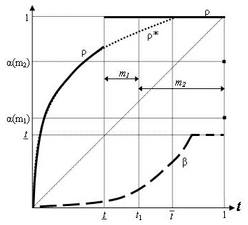
Since the separating function has for all , every LSHP equilibrium displays inflated language, so long as . The inflation of language is inefficient and costly for every type , since such types are revealing themselves in equilibrium, yet not minimizing their message costs. Telling the truth — or more generally, reducing the magnitude of inflation — is not profitable, however, because it would lead to adverse inferences from the Receiver, who expects the equilibrium degree of language inflation and thus rationally deflates (seen in Figure 1 by being strictly below the line).
As mentioned, LSHP equilibria are an intuitively natural class of pooling equilibria to focus on: they feature message monotonicity, which is appealing given the preference of higher types for higher messages; low types separate in the cheapest way possible consistent with message monotonicity; and all pooling occurs on messages in the set , which is effectively the barrier to complete separation. For these reasons, the structure of LSHP equilibria is reminiscent of the “D1” equilibria of Cho and Sobel (1990), the “central pooling” equilibria of Bernheim and Severinov (2003), and, in a more distant setting, the “variable bribes equilibria” of Esö and Schummer (2004).141414A difference with Cho and Sobel (1990) is that there cannot be multiple pools in their D1 equilibria, unlike here where this plays an important role. The difference arises because in the current model, not all types generally wish to be perceived as the highest type, an assumption made by Cho and Sobel (cf. Proposition 1). This is also the case in Esö and Schummer (2004). Multiple pools do arise in Bernheim and Severinov’s (2003) central pooling equilibria; a distinction with their analysis is that it is important here to allow for the possibility that may equal , because there generally will not exist LSHP equilibria with positive when is small. Bernheim and Severinov’s equilibria always have ; the difference stems from the preference distinctions noted in fn. 11. Indeed, Cho and Sobel (1990) established that in standard signaling games where complete separation is not possible due to a bound on the signal space, refinements based on Kohlberg and Mertens’s (1986) notion of strategic stability (Cho and Kreps, 1987; Banks and Sobel, 1987) select equilibria where low types separate in a least costly manner and high types pool on the maximal costly signal. Because the current model has some differences with standard signaling games, these refinements have limited power per se. Nevertheless, Bernheim and Severinov (2003) proposed a modification of the D1 refinement, called monotonic D1 equilibrium, which can be shown to rule out any non-LSHP equilibrium.151515i.e., any equilibrium where the Sender’s strategy is not an LSHP strategy for a positive measure of types. Moreover, there is always an LSHP equilibrium which satisfies the refinement criterion. Therefore, focussing on this class of equilibria can be formally justified. Appendix B provides complete details.
The remainder of this section looks at various special cases of the model which provide additional insights into the structure of communication.
3.3. Large Conflicts of Interest.
LSHP equilibria are particularly simple if the conflict of interest between Sender and Receiver is large in the following precise sense.
Definition 3.
The Sender has (or there is) a large bias if .
When there is a large bias, the Sender would always like to be perceived as high a type as possible, which is the usual assumption in costly signaling games. This implies that there cannot be multiple pools in an LSHP equilibrium, since no type would be willing to send a message if there exists some such that . Consequently, all types above must induce action in equilibrium, and condition (3) becomes vacuous. This yields a simplification of condition (2) and the following result.
Proposition 1.
Assume the Sender has a large bias. There is a single pool in any LSHP equilibrium. It is necessary and sufficient for an LSHP equilibrium with that
| (7) |
have a solution in the domain . It is necessary and sufficient for an LSHP equilibrium with (where all types pool) that
| (8) |
The Proposition implies that if there is large bias, then for any , there is at most one message in that is used in an LSHP equilibrium. Therefore, the rich language assumption that be large for each is unnecessary; the analysis would apply just as well if instead for all . Note also that it is simple to directly establish existence of an LSHP equilibrium under large bias.161616The argument is as follows: if (8) does not hold, then there must be at least one solution to , since each side of is continuous, and at the right-hand side is whereas the left-hand side is strictly positive (by and large bias). This is because the only binding incentive constraint is for type , unlike in the general bias case where incentive constraints can also bind for boundary types between pools.
3.4. No Conflict of Interest.
I have assumed that for all , which was crucial for Theorem 1. At the other extreme, consider for all , so that there is no conflict of interest. Intuitively, one would expect complete separation with truth-telling in this case. Formally, although (DE) does not apply, it is clear that the appropriate separating function becomes for all . There is a separating equilibrium where each sends any , with the caveat that any and use distinct messages if . Since in such equilibria, these are indeed LSHP equilibria.
3.5. Almost-Cheap Talk.
Return now to the general case of conflict of interest. Recall that when , the setting reduces to the CS model of cheap talk. An interesting question then is what happens when the intensity of lying cost is small, . It must be that in any LSHP equilibrium, because by (DE), the separating function cannot be extended very far, i.e. . Hence, as the cost of lying vanish, the type space is almost entirely partitioned into pools, with extremely inflated language.171717 Since (3) must hold for every boundary type in the partition of , and , the partition of must be close to some CS partition in any sensible metric. Chen et al. (2008) discuss which cheap-talk equilibria can be limits of a class of equilibria in a model of costly lying as the lying costs vanish. Although their model does not nest the current setting, and the class of equilibria they consider does not include all LSHP equilibria (they require monotonicity of the Receiver’s strategy, which need not hold in an LSHP equilibrium), one can nevertheless show that if is strictly increasing, any cheap-talk equilibrium which is the limit of a sequence of LSHP equilibria as must satisfy Chen et al.’s (2008) No Incentive to Separate property. The following result says that in fact, there generally is an LSHP equilibrium where no type separates.
Proposition 2.
Assume that there is no CS cheap-talk equilibrium, , with . Then, for all sufficiently small, there is a LSHP equilibrium with , where types partition as in a CS cheap-talk equilibrium.
The assumption made in the proposition is mild: intuitively, it holds “generally” in the sense that if a given constellation of , , and (the prior on types) has a cheap-talk equilibrium with , then small perturbations to any of the three functions would lead to the assumption being satisfied.181818For example, in the uniform-quadratic case of CS, which is parameterized by a single number that measures the magnitude of conflict of interest, the assumption only excludes , which is a nowhere-dense set of zero Lebesgue measure. The proof uses a result from Chen et al. (2008) that there is always a cheap-talk equilibrium where , under the assumption. Pick any one of these; if is sufficiently small, then it is an LSHP equilibrium for all types to pool just as in the cheap-talk equilibrium, using messages only in , with the Receiver responding to any with .
3.6. Very Costly Talk.
Consider what happens as the intensity of lying cost, , gets large. A simple observation is that the possible gains from lying for any type are bounded in a PBE, since the range of the Receiver’s strategy in a PBE is contained in . Hence, for any and any , any PBE satisfies if is sufficiently large. Since the type space is compact, it follows that when is sufficiently large, any PBE is close to truth-telling. Consequently, in a LSHP equilibrium, becomes arbitrarily close to as . This implies that when all types have distinct cost-minimizing messages (so that is strictly increasing), there is just a single pool in an LSHP equilibrium when is sufficiently large, since all types sufficiently close to wish to be perceived as high a type as possible.
4. An Example and Application
To complement the somewhat abstract analysis thus far, this section works out a canonical example, providing some further analysis that may be useful for applications. I then apply the results to the question of communication versus delegation (Dessein, 2002).
4.1. Example.
The example is based on the uniform-quadratic setting of CS that has been the workhorse for applied work: , , and for some bias parameter . For the lying cost structure, assume that and .191919It is not important what the message space is, so long as it satisfies the maintained assumptions. For concreteness, one can suppose that for each , , so that . As discussed in Section 2.1, this has the interpretation that the Sender’s message has two components: he reports an exact value about his type (which bears a lying cost) and a cheap-talk message. In other words, the Sender’s lying cost is quadratic in the distance between his true type and the type he claims to be. This specification satisfies all the maintained assumptions and, as will be seen, is tractable. It implies that , , , and .
The quadratic lying cost permits a closed-form solution for the separating function, . To derive it, first observe that the differential equation (DE) can be simplified to
| (9) |
The reader may verify that the family of solutions to (9) is given by
| (10) |
where is a constant to be determined. Since the separating function has the initial condition , it follows from (10) that . Substituting this value of into (10) and manipulating terms yields the following solution for the separating function:
| (11) |
The upper bound on types that can separate using , defined by , can be solved for explicitly from (11) as
| (12) |
It is straightforward to check that because and , , as predicted by Theorem 1. Moreover, is increasing in and converges to (resp. 1) as (resp. ). This confirms the intuition that the maximal feasible set of separation, , is larger when the cost of lying is larger relative to the conflict of interest.
The necessary conditions for LSHP equilibrium, (2) for the boundary types between pools and (3) for , can be simplified for the current setting as follows:
| (13) | |||
| (14) |
Note that condition (13) is the well-known form that CS’s arbitrage condition takes under uniform prior and quadratic preferences. Theorem 2 also implies that there is an LSHP equilibrium that satisfies
| (15) |
This condition says when there are no separating types, type weakly prefers pooling with and incurring message cost (the cost of sending any message in for type ) to revealing itself at no cost. Conversely, given any solution to (13)–(15), there is a corresponding LSHP equilibrium.
The next result focuses on LSHP equilibria with a single pool, for these are particularly tractable and permit clear comparative statics. Condition (13) is vacuous in this case, and conditions (14) and (15) are simplified by setting .
Proposition 3.
In the leading example:
-
(a)
A single-pool LSHP equilibrium exists if and only if , or equivalently,
(16) In particular, a single-pool LSHP equilibrium exists if either or .
-
(b)
A single-pool LSHP equilibrium with (i.e., an uninformative LSHP equilibrium) exists if and only if .
-
(c)
All single-pool LSHP equilibria are essentially equivalent, i.e. they have the same cutoff type .
-
(d)
If , all LSHP equilibria have a single pool and are essentially equivalent.
-
(e)
Fix any and let denote the cutoff in single-pool LSHP equilibria as a function of , defined on some interval given by (16). Then is continuous and increasing, strictly increasing at any with , and differentiable at all .
The Proposition has a number of interesting implications. Key is part (c), which assures that all single-pool LSHP equilibria have the same cutoff, and hence are essentially or outcome equivalent. CS showed that under cheap talk, an informative equilibrium — one where no Receiver action has ex-ante probability one — exists if and only if . Part (d) of the Proposition implies that when cheap talk cannot be informative, all LSHP equilibria are essentially equivalent and have a single pool, although they are not necessarily uninformative. Indeed, combining parts (a), (b), and (d), we see that for any positive lying cost intensity, there is a set of biases for which there would be no informative cheap-talk equilibrium but there is an informative and essentially unique LSHP equilibrium. Part (b) of the Proposition also implies that if there is an informative cheap-talk equilibrium (), all LSHP equilibria are informative. Furthermore, part (a) of the Proposition implies that when cheap talk can be informative, there is a threshold such that for all , there is a single-pool LSHP equilibrium, whereas for all , every LSHP equilibrium has multiple pools.202020It can also be shown that for any , if is small enough, every LSHP equilibrium has exactly pools, where is the maximal number of actions that can be induced in a cheap-talk equilibrium with bias . CS showed that is the smallest integer greater than or equal to The last part of the Proposition provides a comparative static on single-pool LSHP equilibria: in particular, for any , the unique cutoff is strictly increasing in when the cutoff is strictly positive. Hence, when the lying cost intensity increases, single-pool LSHP equilibria become more informative (when they exist) in the strong sense of refining the Receiver’s information partition.
4.2. Application: Communication versus Delegation.
Dessein (2002) raised the question of whether the Receiver can do better by delegating decision-making to the Sender, without any constraints, rather than communicating via cheap talk with him. The tradeoff is one of “loss of information” under communication versus “loss of control” under delegation. Dessein proved that which arrangement is better for the Receiver depends upon the magnitude of conflict: delegation is superior to cheap-talk communication if and only if the agent’s bias is sufficiently small. In particular, in the uniform-quadratic setting of CS that is the focus of this section, delegation is preferred whenever cheap talk can be informative, i.e. whenever the bias is .
The results derived in this paper so far suggest that when manipulating information may have some costs, whether delegation dominates communication or not will depend upon the cost intensity. The discussion in Section 3.6 implies that for any given conflict of interest, communication strictly dominates delegation when is large enough, even though there is always some loss of information under communication. The more subtle and interesting question, though, is whether for every finite intensity of lying cost, delegation will dominate communication for all small enough conflicts of interest. The issue is important for understanding whether the central organizational tradeoff identified by Dessein — loss of information versus control — remains relevant so long as information is at all manipulable.212121If information is not manipulable at all, or equivalently there are infinite lying costs, then as Dessein (2002, p. 831) noted, communication will be fully revealing and hence dominate delegation for all levels of bias.
For the parametric setting of this section, I am able to provide a sharp negative answer. Following Dessein (2002), say that communication is superior to or dominates delegation if there is an equilibrium under communication in which the ex-ante welfare of the Receiver is strictly higher than under delegation.
Proposition 4.
In the leading example, there is a finite such that for any , communication is superior to delegation for all . In particular, if and , communication is superior to delegation.
To gain some intuition for the result, note that by the earlier discussion, the key issue is whether there exists some cost intensity for which communication dominates delegation for all small enough biases. The answer is a priori unclear because, for any fixed level of lying cost (including cheap talk), both communication and delegation approach the first best as conflicts vanish. Dessein (2002) showed that delegation is an order of magnitude superior to cheap-talk communication when conflicts are small. This implies that since LSHP equilibria for any have one or more interval pools on the highest messages, delegation will be superior to communication if the set of pooling types is too large relative to the bias. Therefore, for communication to dominate delegation requires that the region of separating types be large enough relative to the bias. The proof of Proposition 4 shows that this is the case in single-pool LSHP equilibria for the relevant parameters.
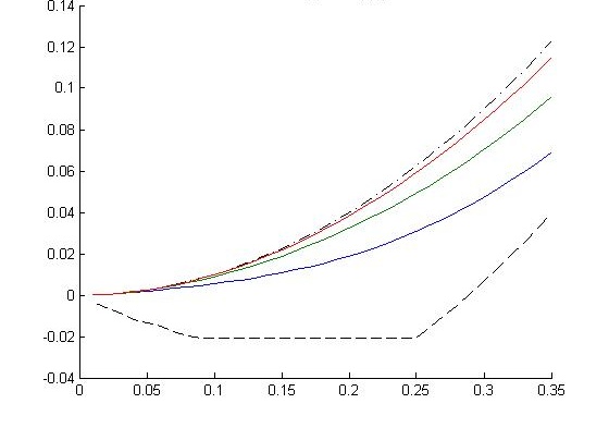
How large exactly must lying costs be in order for communication to dominate delegation for all biases? Numerical analysis reveals that is sufficient; recall from Proposition 3 that this is precisely the threshold cost intensity that guarantees existence of single-pool LSHP for all . Figure 2 graphs the difference in the Receiver’s ex-ante utility from communication over delegation as a function of for different values of . The figure shows that for any , communication is superior to delegation for any . As , communication becomes close to fully revealing (which yields ex-ante utility to the Receiver), hence the Receiver’s welfare difference between communication and delegation converges to (which is the Receiver’s utility under delegation).
5. Withholding Information and Verifiable Disclosure
The cheap-talk approach to strategic communication assumes that it is costless for the Sender to lie arbitrarily. An alternative approach, initiated by Grossman (1981) and Milgrom (1981), is to assume that that the Sender can tell the truth or withhold information at no cost, but cannot lie. A justification is that “there are penalties for perjury, false advertising or warranty violation that are sufficiently sure and heavy that false reporting never pays” (Milgrom and Roberts, 1986b, p. 19). In the literature, this is often referred to as verifiable disclosure, or persuasion or partial-provability. The classic result is that there is complete separation in every PBE (Seidmann and Winter, 1997), due to a well-known “unraveling argument.”222222In general, unraveling requires enough structure on preferences — satisfied by the CS assumptions on and — and that each type be able to verifiably disclose itself if it wishes to. This is in striking contrast with the cheap-talk prediction of no information revelation when there is a large enough conflict of interest between Sender and Receiver (Crawford and Sobel, 1982, Corollary 1).
Costly lying provides a framework to unify these divergent results. However, the basic model I have studied has a limitation in this respect: it does not permit the Sender to withhold information freely, and to this extent, the model does not perfectly correspond to verifiable disclosure when . Accordingly, this section develops an extension to accommodate the costless withholding of information.232323I am grateful to Yeon-Koo Che for prompting this extension.
5.1. A Simple Form of Withholding Information.
For this section, assume that and that , to provide a clear comparison with the standard verifiable disclosure setting. Moreover, to avoid some tedious complications that do not add much insight, assume that the Sender always wishes to be thought of as the highest type, i.e. there is large bias. This is the standard assumption in verifiable disclosure models, and as noted above, implies that cheap talk and verifiable disclosure generate polar predictions.
Augment the message space to now be , where is as before, and is a new set of one or more messages (i.e., and ). Assume that for any and , ,242424Writing involves an abuse of notation, but is a convenient shorthand that should not cause any confusion. so that all messages in are equally costly for the Sender. The rest of the model remains as before. The set can be viewed as a set of pure cheap-talk messages (it is without loss of generality to normalize for all and ), or as the Sender being silent, or otherwise freely withholding information.252525If one instead assumes that for any and , then the Sender’s cost of sending any has fixed and marginal components. Although this formulation is not analyzed here, I note that when combined with “,” it yields a model akin to costly disclosure (e.g., Verrecchia, 1983), which has also been studied recently by Esö and Galambos (2008). In this formulation, withholding information takes a particularly stark and simple form: at the limit as , the Sender is effectively choosing between either credibly revealing his true type, or sending a message that is costless to all types. While this structure will be generalized shortly, it is convenient to start with this simple formulation, which I call the withholding model.
Consider first whether there can be full separation for any . Suppose there is such an equilibrium. Any message in can not be used by any , for all lower types would mimic it. This implies that separation of all types greater than zero must be achieved with non-withholding messages. However, the argument of Theorem 1 can be extended to show that this is impossible. Consequently, there must be pooling in equilibrium. As it is not my goal to characterize every pooling equilibrium, some of which can be implausible,262626For example, there is always an uninformative equilibrium where all types send the same , and the Receiver responds to every message with . This can be ruled out by standard refinements such as Cho and Kreps’s (1987) D1 criterion, for any (and even weaker criteria for large ). I only show that LSHP equilibria can be extended in an obvious way to the current environment.
To state this precisely, start with any LSHP equilibrium strategy profile when withholding is not allowed. Now consider a strategy profile in the withholding model where the Receiver responds to any withholding message, , with a maximally skeptical inference and plays ; in other respects, strategies are identical to the LSHP profile. Call such a strategy profile an augmented LSHP profile.
Proposition 5.
An augmented LSHP profile is an equilibrium of the withholding model.
The reason is simple: given the Receiver’s play, telling the truth is always at least as good (strictly better if ) as withholding, since it costs the same and leads to a weakly preferred (strictly, if ) action. Hence, for any lying cost intensity, arbitrarily large or small, there are equilibria with the following properties: there is lying on the equilibrium path (since a positive measure of types play in any LSHP equilibrium); there exists some such that types in form a single pool, claiming to be the highest type; all types below separate, but claim to be higher types than they truly are; withholding does not occur on the equilibrium path; and the Receiver responds to withholding with a maximally skeptical inference. These last two properties are standard in the equilibria of verifiable disclosure games (e.g., Milgrom and Roberts, 1986b, Proposition 2), with the caveat that of course the lowest type could just as well fully disclose or withhold.
Proposition 5 implies that the insights of the original non-withholding model can be applied to the current environment. Of particular interest are the limits as or .
Corollary 1.
When , any equilibrium in an augmented LSHP profile is uninformative, with all types pooling on some . As , any sequence of equilibria in augmented LSHP profiles has and, for all , .
Thus, at the cheap-talk limit of augmented LSHP equilibria, not only is there no information revealed,272727Note that since bias is assumed to be large, all cheap-talk equilibria are uninformative. but language is entirely inflated (all types claim to be the highest), whereas at the verifiable disclosure limit, there is full separation through truth-telling. In this sense, the augmented LSHP equilibria provide a sensible spanning of the extreme cases both in terms of how much information is conveyed and the messages that are used.
5.2. Richer Forms of Withholding.
As previously noted, the withholding model discussed above is special because, at the limit of , the Sender has only two undominated choices: either completely withhold information about his type or completely reveal it. Verifiable disclosure models often endow the Sender with a much richer set of choices, such as reporting that his type lies in any closed subset of the type space that contains his true type. This is meant to capture the idea that the Sender can credibly reveal some information without revealing it all. To consider such possibilities when lying costs are not infinite requires a specification of the cost of each such message for each type. I will discuss a simple formulation which allows the previous analysis to extend.
Let be any set of closed subsets of , such that as for each , . The Sender is permitted to claim that his type lies in any element of , i.e. for any , there is a (non-empty) set of messages with the literal meaning “my type is in .” Let be any function satisfying and if . Starting with the usual cost function that is defined for all precise statements (i.e., any singleton ), I extend it to each vague statement (i.e., any non-singleton ) by assuming that for any , . That is, the cost for the Sender of claiming that his type is in a set is the same as the cost of claiming that his type is exactly . Note that by the assumed properties of , the cost for any type of claiming to be in any set is the same as the cost of claiming to be if and only if .282828The assumptions on can be weakened to relax this implication, but it would unnecessarily complicate the subsequent analysis.
The model without any withholding is the special case where consists only of singleton sets. The withholding model discussed earlier is the case where consists of just the singletons and the set , with for all . In general, one natural possibility for is that . This captures the idea that a vague statement is a lie to the extent it is a lie when given its most favorable interpretation, i.e. the distance of the true type to the closest point in . For any , the Sender’s undominated choices at the limit of are to claim that his type is in any such that , which is precisely any such that , just as in standard disclosure models.
The key to extending LSHP equilibria to this setting, for any lying cost intensity, is to have the Receiver respond to any message with the most skeptical inference among the set of types for whom that message is least costly. Formally, pick any LSHP equilibrium profile when withholding is not available that satisfies if and for two types . (Such an LSHP equilibrium profile exists by the proof of Theorem 2.) The profile specifies the Receiver’s response, , for any with . Extend to vague messages as follows: for any with , for some . In other words, if the Sender claims to be in a non-singleton set , the Receiver responds by taking some action that she would in response to a claim that the Sender is the lowest type in .292929The reader may wonder why not use a simpler construction where the Receiver plays if with . The reason is that even though this simpler construction will also be an equilibrium, it will not satisfy standard refinements (such as the D1 criterion) for all . In particular, as , it requires the Receiver to form the implausible belief that the Sender is type upon observing any vague message, even if it is prohibitively costly for type 0 to send that message. The construction in the text is not vulnerable to this objection; rather, beliefs as converge to equilibrium beliefs of the verifiable disclosure game. To see that this extended LSHP profile is an equilibrium for any , suppose to contradiction that is a profitable deviation for a type . By construction, there exists such that . If , , hence is a profitable deviation, a contradiction since we started with an LSHP equilibrium profile. If , then any is a profitable deviation, because and , also a contradiction since we started with an LSHP equilibrium profile.
6. Conclusion
This paper has studied a model of communication between an informed Sender and an uninformed Receiver, where the Sender has a cost of lying or misrepresenting his private information in certain ways. These costs on the Sender may stem from various sources, such as technological, legal, or psychological constraints. The main results show that inflated language naturally arises in this environment, where the Sender (almost) always claims to be a higher type than he would under complete information. Regardless of the intensity of lying cost, there is incomplete separation, with some pooling on the highest messages. How much information is revealed is a function of the intensity of lying cost. An extension of the basic model to allow costless withholding of information provides a unified framework to embed both cheap talk and verifiable disclosure as limiting cases.
The basic finding that lying costs enlarge the scope for direct communication to reduce the costs of asymmetric-information-based incentive problems is, on one hand, not surprising, but on the other hand, likely important in a wide variety of economic problems. A formal framework and analysis such as that developed may be useful in applications where it is important to understand exactly how incentive constraints are relaxed.
Section 4 provided one such example, focussing on the interaction between preference conflicts and lying costs. In an influential paper, Dessein (2002) argued that when a decision-maker or principal is faced with a biased but better-informed agent, unconstrained delegation of decision-making is better than cheap-talk communication whenever the conflict of interests are not too large. I have shown that in the simple but canonical setting of Section 4, if misrepresentation costs are even moderately large, this conclusion is reversed: the principal prefers to communicate than delegate regardless of how small the conflict of interest is, even though communication necessarily entails some loss of information. Besides matters of generalization, this raises a number of substantive questions. For example, Ivanov (2007) has shown that the principal is better off restricting the precision of the agent’s information compared to either delegation or cheap-talk communication. Plainly, the magnitude of misrepresentation costs will have a significant effect on how beneficial such “information control” is. In the limiting case of verifiable information or infinite lying costs, the principal would strictly prefer to not restrict information at all. Whether information control is valuable whenever lying costs have finite intensity, and if so, how this control should be structured are open questions.
The fact that lying costs can mitigate inefficiencies resulting from asymmetric information suggests that applications to negotiation and bargaining will also be fruitful. For example, Valley et al. (2002) document striking experimental evidence that subjects in double auctions achieve greater efficiency given pre-play communication than the theoretical limits derived by Myerson and Satterthwaite (1983).303030I thank Vince Crawford for this reference. Importantly, the subjects do significantly better when communication is face-to-face than through written messages, which Valley et al. (2002) largely attribute to their evidence that subjects misrepresent valuations substantially less in face-to-face communication than in written messages. It seems plausible that the more direct the interface of communication, the more costly (difficult, uncomfortable, etc.) it is to lie. Accordingly, these empirical findings may be organized by a framework such as that developed here, although a model adapted to the bargaining environment would yield more finely-tuned insights.
Appendix A: Proofs
Proof of Lemma 1. By hypothesis, types are separating in a monotone PBE with mapping . If is constant on some interval , then some can profitably deviate and mimic a slightly higher type , contradicting equilibrium separation; hence must be strictly increasing on . This implies that for any , . Separation requires that for each , must be a solution to (1). If is differentiable on , then the first order condition obtained by differentiating (1) is (DE), as required. So it suffices to prove that is differentiable on . This is done in series of steps.
Claim: for all .
Proof: Suppose there exists a such that . Without loss, we can assume that , because otherwise cannot be strictly increasing on . This implies that
| (A-1) |
Define as the expected utility gain for a type by deviating from to . Since we are on a separating portion of the type space when is small,
Since ,
is differentiable in a neighborhood of , and has derivative
Observe that and (using (A-1)). Hence, for small , , implying that a type strictly prefers to imitate , contradicting equilibrium separation of .
Claim: for all .
Proof: Suppose not. By the previous Claim, there exists a such that . By monotonicity of , for all . It follows that for small enough , . On the other hand, for small enough , . Therefore, for small enough , a type strictly prefers to imitate , contradicting equilibrium separation of .
Claim: is continuous on .
Proof: Suppose there is a discontinuity at some First assume . By the continuity of and , and the monotonicity of , as ,
where the inequality above follows from . On the other hand, as ; hence, for small enough , prefers to imitate , contradicting equilibrium separation.
The argument for the other case where is similar, establishing that prefers to imitate for small enough .
Claim: is differentiable on .
Proof: Given the previous claims that is continuous
and does not intersect on , one can replicate the argument of Mailath (1987, Proposition 2 in
Appendix).
∎
The following Lemma is used in the proof of Theorem 1 and proves uniqueness of the separating function.
Lemma A.1.
Fix any . There is a unique solution to the problem of finding a and such that (i) is strictly increasing and continuous on , (ii) , (iii) solves (DE) on , and (iv) if . Moreover, if , otherwise .
Proof.
If , the Lemma is trivial, so assume . Since for all such that , there is no Lipschitz condition on (DE) on the relevant domain, in particular even locally if . Thus, standard results on differential equations do not apply. Instead, I proceed as follows, building on Mailath (1987).
Step 1: (Local existence and uniqueness.) Consider the inverse initial value problem to find such that:
| (A-2) |
By the assumptions on , , and , is continuous and Lipschitz on . Hence, standard theorems (e.g. Coddington and Levinson, 1955, Theorem 2.3, p. 10) imply that there is a unique location solution, , to (A-2) on , for some ; moreover, .313131 is the set of all Real-valued functions on that have a continuous derivative at all and in addition have a right-hand derivative at that is continuous from the right at . Inverting gives a strictly increasing on such that , solves (DE) on , and . Note that for all . Since the inverse of any increasing local solution to (DE) is a local solution to (A-2) on for some , local uniqueness of an increasing solution to (DE) follows from the fact that is the unique local solution to (A-2) above .
Step 2: ( is bounded away from above .) Suppose is a solution to (DE) on , with and . Let . I claim that . This is obviously true if , so assume , and , towards contradiction. We must have (because for all ) and . Let . By the assumptions on , . Since , there exists such that for all . Pick such that . We have
which contradicts .
Step 3: The proof is completed as follows. If is defined on with , then by the previous step, is continuous, Lipschitz, and bounded in a neighborhood of , hence standard theorems (e.g. Coddington and Levinson, 1955, Theorem 4.1 and preceeding dicussion, p. 15) imply that there is a unique extension of to for some ; this extension is strictly increasing, in , and by the previous step, . Now let . Clearly, . Moreover, we must have , for otherwise can be extended beyond . We are done by setting . ∎
The following Lemma is used in the proof of Theorem 2.
Lemma A.2.
Proof.
The proof is constructive.
Step 0: Preliminaries.
Start by defining the function
is the utility gain for type from sending a message in and receiving its ideal action over separating itself (thus inducing ) with a message in . Note that in an LSHP equilibrium, the gain from pooling over separating can be no more than , and will generally be strictly less. There are two conceptually distinct cases: one where for some , and the other where for all . Define
is continuous and ; hence and for all , . In everything that follows, we are only concerned with . So statements such as “for all ” are to be read as “for all ” and so forth unless explicitly specified otherwise.
Step 1: Constructing the necessary sequences.
Initialize and . Define
Clearly, is continuous in both arguments, and strictly concave in with a maximum at . Since for all , it follows that for any such , in the domain there exists a unique solution to . Call this . Similarly, on the domain there exists a unique solution to . Call this . By continuity of , and are continuous, , and if By the monotonocity of , for and , there is either no solution or a unique that solves . If there is a solution, call it , otherwise set . It is straightforward that and are continuous functions, with equality if and only if , and . Note that , and if .
For and recursively define as the solution to
if a solution exists that is strictly greater than , and otherwise set . By the monotonicity of and , is well-defined and unique. Define . Note that for all , and if and only if . For all and , is continuous, for all , if , and (these follow easily by induction, given that we noted all these properties for ).
Step 2: The critical segment B.
I claim there exists such that . (Obviously, if it exists, it is unique.) To see this, first note that by definition, . Let .323232Recall that the infimum of an empty set is . It is sufficient to show that such that for any , . By construction, and . Since , we are done.
Step 3: Existence when .
Consider the functions and . These are continuous, and . Moreover, ; hence either or . It follows that there is some type such that either (i) and for all ; or (ii) and for all . Let if (i) is the case; if (ii) is the case. By construction, setting and for satisfies the needed properties.
Step 4: Existence when .
By the continuity of and , the logic in Step 3 can fail when only if . So suppose this is the case. Note that this requires . For any , , with strict inequality for interior . In words, when , type weakly prefers (indifference at the endpoints and strict preference for interior ) inducing with a message in over inducing with message in . This follows from the construction of and , and . Given any , define , , and recursively, for , as the solution to
if a solution exists that is strictly greater than , and otherwise set . It is straightforward that for all , is continuous in . Since , it follows that is well-defined and lies in . By construction, setting and for satisfies the needed properties.
Finally, the proof of the Lemma is completed by noting that for all large enough if , because if and for all large enough in this case. ∎
Proof of Theorem 2.
The necessity of (4) and (5) follows from the discussion in the text preceding the Theorem. Fix any and a strictly increasing sequence that satisfy conditions (4), (5), and (6). I will show that there is a corresponding LSHP equilibrium. This suffices to prove the Theorem because of Lemma A.2.
I first define the strategy profile. Based on the discussion in the main text preceding the Theorem, the Sender’s strategy, , is clear, with the only possible ambiguity being for types : assume for concreteness that they “pool up” rather than “down” (so type does not separate). Let be the set of messages used in this strategy. It is clear what the Receiver’s response, , must be for any . For any , the Receiver plays as follows:
-
(1)
For any with , .
-
(2)
For any with , .
-
(3)
For any with , .
-
(4)
For any , .
I now argue that as constructed above is an LSHP equilibrium. Obviously, is an LSHP strategy and is optimal given beliefs that are derived by Bayes rule on the equilibrium path. So it only needs to be shown that is optimal for the Sender.
No type has a profitable deviation to some , because for any and for all since (3) holds for each () and . This logic also implies that if any has a profitable deviation to some , it has a profitable deviation to some . Note also that if any type has a profitable deviation to some where , then it has a profitable deviation to some , because is cheaper than for all types, and they both lead to the same action, .
Claim: Assume . Then no type has a profitable deviation to any .
Proof: By Lemma A.2, type does not have a profitable deviation to any . So I prove the result by showing that if some type has a profitable deviation to some , then type has a profitable deviation to . For this, it suffices to show that if and , then
Fix a and . Since , we have
and hence it suffices to show that
This inequality can be rewritten as
which holds because .
Claim: Assume . Type is indifferent between playing and playing any , but strictly prefers to any . Any strictly prefers to any .
Proof: The indifference property for type is proved by two observations: if , then it is immediate from Lemma A.2 and that for all ; on the other hand, if , then for any , and and have the same cost. Note that if , Lemma A.2 implies that .
Equation implies that for all ,
Since , this implies that for any ,
Therefore, by continuity, any strictly prefers to any .
To show that any strictly prefers to any , pick any such . The highest utility for when constrained to sending is attained by sending . From the previous arguments,
and hence it suffices to show that
| (A-3) |
Since (A-3) is true if
which can be rewritten as
which holds since .
The argument for types strictly preferring to any is analogous to above.
Claim: Assume . No type has a profitable deviation to any .
Proof: The result is vacuously true if , so assume that . Any is responded to with , hence when constrained to such messages, any type maximizes utility by sending an , because . However, by the previous Claim, all weakly prefer playing to any . This proves the claim for any .
To prove the claim for all , it suffices to show that if has a profitable deviation to an , then type has a profitable deviation to , since the latter is not possible. To prove this, it suffices to show that for any and ,
Fix a and . Since , it suffices to show that
This is true if
which can be be rewritten as
which is true because .
The above claims establish that is optimal for the Sender,
completing the proof.
∎
Proof of Proposition 1. Large bias implies that for any , is strictly increasing on . Hence there cannot be multiple pools in an LSHP equilibrium because all pools use messages in , imposing the same direct message cost on any type, whereas higher actions are strictly preferred by all types.
Necessity of (7) for is straightforward, since if it does not hold, continuity implies that for small enough , either some type will deviate from to , or will deviate from to . Sufficiency of (7) with for an LSHP equilibrium follows from the observation that such a and (trivial) sequence satisfies and (4) and (5), and therefore the equilibrium construction of Theorem 2 applies.
Proof of Proposition 2.
Chen et al. (2008, Proposition 1) show that
there is always a strictly increasing sequence such that for
, satisfies (3), and
moreover, . Under the
Proposition’s assumption, we cannot have . This implies that for all sufficiently small
enough, the sequence combined with satisfies (4) and
(6), and therefore the equilibrium construction of
Theorem 2 applies.
∎
The following Lemma is used in the proof of Proposition 3; it shows that when increases, the separating function decreases pointwise.
Lemma A.3.
Assume . Fix , and let and denote the separating function when and respectively, with respective domains and . Then and for all , .
Proof.
Since , Lemma A.1 implies that and . It suffices to show that for all , because then and Lemma A.1 implies that . Suppose, to contradiction, that for some . For any , (DE) implies that if , then . Consequently, we must have for all . This implies that for all , . Reformulating in terms of inverse functions, we have that for all , , yet and for . This contradicts the Fundamental Theorem of Calculus applied to and . ∎
Proof of Proposition 3. (a) Equation (12) and simple algebra shows that is equivalent to (16). It is obvious that (16) is satisfied if ; to see that it is also satisfied if , let and compute that when , , , while .
Now suppose . If , then and satisfy (6), and we are done. So assume . A little algebra shows that . By continuity, there exists that satisfies (14). This and satisfy (5), and we are done.
Now suppose . Simple algebra shows that for any , , hence (14) cannot be satisfied with any and . So all single-pool LSHP equilibria must have , inducing the Receiver to play in equilibrium. Since requires , type strictly prefers any action in to . Consider any for . If , type has a profitable deviation to since it weakly prefers to action and strictly saves on lying cost. So, . But then, type has a profitable deviation to because it strictly prefers to and saves on lying cost. Consequently, there are no LSHP equilibria.
(b) A single-pool LSHP equilibrium with exists if because in this case, , hence and satisfy (6). If , then the argument used in part (a) to show that there is no uninformative LSHP equilibrium applies.
So it remains to show that there is no uninformative LSHP equilibrium when . Suppose, to contradiction, that there is. Consider any . Let be the Receiver’s response to . Type not deviating to requires . Since , we must have
| (A-4) |
which implies that , since . On the other hand, type not deviating to requires , which implies that
| (A-5) |
We have a contradiction between (A-4) and (A-5) if
which simplifies after some algebra to , which holds since and .
(c) If , the statement is vacuously true because there are no single-pool LSHP equilibria by part (a). If , simple algebra shows that for all . By part (b), there is no single-pool LSHP equilibrium with , and by the necessity of (14) for any LSHP equilibrium, there is no single-pool LSHP equilibrium with either. Therefore, by part (a), all LSHP equilibria have cutoff .
It remains to consider . Define
| (A-6) | |||||
| (A-7) |
By (14), there is a single-pool LSHP equilibrium with strictly positive cutoff if and only if for some ; by part (b), there is one with cutoff if and only if . Taking derivatives yields , , , and , where the derivatives of have been simplified using the fact that solves (9). Thus, . Since implies , we conclude that there is at most one solution to on the domain . Moreover, if and only if there is no solution to with , yielding the the desired conclusion.
(d) When , there cannot be multiple pools in an LSHP equilibrium because (13) will be violated. Furthermore, all single-pool LSHP equilibria are essentially equivalent because implies , and the rest of the argument of part (c) applies.
(e) Fix any any such that (16) is satisfied. In what follows, I add as an argument to various objects to emphasize the dependence on the cost intensity. First consider . By part (b), for all in a neighborhood of , hence .
Now consider . Then for all in a neighborhood of , where and are defined in equations (A-6) and (A-7) (note that does not depend on ). It is routine to verify that for any , is continuous on the domain of for which is well-defined. This implies that for any , is continuous on the domain of for which it is defined. Hence is continuous at . Next I argue that it is strictly increasing and differentiable at . By the Implicit Function Theorem,
| (A-8) |
so long as the denominator is non-zero, which will be shown below. The numerator of the right hand side of (A-8) computes as
which is strictly positive because and by Lemma A.3 (that the derivative exists is routinely verified). To sign the denominator, note that for all by the calculation performed in part (c). Hence, if , we would have because , which implies that since . But this is impossible because by (A-6), for all , and by part (a). Consequently, the denominator of the right hand side of (A-8) is strictly positive. Therefore, .
Finally, consider . Then by part (b),
, hence is left-continuous at
. Since holds for all , the continuity argument used above implies that
is also right-continuous at .
∎
Proof of Proposition 5.
Since on-path behavior in an augmented LSHP profile is identical to
an LSHP equilibrium, I only need to verify that deviating to some
is not profitable for any type. Fix any type and
some . Since the (non-augmented) LSHP profile is an
equilibrium, it is not profitable for type to deviate some
unused , which induces an action
. But then, since all cost the same as , and by large bias,
, deviating to is not
profitable for type .
∎
Proof of Corollary 1. Since bias is large, Proposition 1 implies that if , (7) must hold. But the left-hand side of (7) is bounded above zero on the domain for any set of that is bounded away from ; whereas the right-hand side is converging to as . Hence, for small enough , there is no solution to (7) in the domain , which proves the first part of the Proposition.
The second part follows from the discussion in Section
3.6, noting that since
in the withholding model.
∎
Proof of Proposition 4. I will show that for and , there is an equilibrium under communication in which the Receiver’s ex-ante utility is strictly higher than , which is her utility from delegation. This proves the Proposition because by the discussion in Section 3.6, for all , communication is arbitrarily close to fully-revealing and hence dominates delegation for all large enough . For all , communication dominates delegation for any , because even an uninformative equilibrium under communication yields ex-ante utility to the Receiver strictly greater than .
Accordingly, assume and . By Proposition 3, there are single-pool LSHP equilibria for these parameters. R’s utility in a single-pool LSHP equilibrium with cutoff is , since all types below separate and all types above form a single pool. Hence this equilibrium yields higher utility than delegation if
or equivalently,
| (A-9) |
Proposition 3 implies that (because for all ), hence (A-9) holds if
which is true because .
∎
Appendix B: Equilibrium Refinement
This appendix develops a rigorous justification for focussing on LSHP equilibria, by applying an equilibrium refinement proposed by Bernheim and Severinov (2003) called the monotonic D1 (mD1) criterion. The first part below explains and formalizes the criterion; the second part applies it to the current model, deriving the sense in which it justifies LSHP equilibria.
The Monotonic D1 Criterion
The underlying idea of the mD1 criterion is the same as Cho and Kreps’s (1987) D1 criterion, which requires that the Receiver not attribute a deviation to a particular type if there is some other type that is willing to make the deviation for a strictly larger set of possible Receiver responses. The mD1 criterion strengthens this by applying the test to only those responses from the Receiver which satisfy an action monotonicity restriction. Analogous to message monotonicity for the Sender, action monotonicity requires the Receiver’s strategy to satisfy if . In words, if the Sender claims to be a strictly higher type, the Receiver should respond with a weakly higher action. Intuitively, given message monotonicity, action monotonicity is natural (and indeed, is an implication of message monotonicity on the equilibrium path).
Some notation is needed for the formal statement. With respect to a given profile , which induces some , define
where I follow the convention that and . To understand these functions, suppose is an equilibrium with message and action monotonicity. If some type claims to be on the equilibrium path, then (resp. ) is just the “lowest” (resp. “highest”) equilibrium action taken in response to a claim of . If no type claims to be , yet some type does claim to be a (resp. ), then (resp. ) is the “highest” (resp. “lowest”) action taken by the Receiver in equilibrium to a claim of being lower (resp. higher) than . If no type claims to be any (resp. ), then (resp. ) just specifies the lowest (resp. highest) rationalizable action for the Receiver.
With respect to some profile , let
To interpret, consider an unused message in some equilibrium. (resp. ) is the set of responses within the set that give type a weak (resp. strict) incentive to deviate to .
The following is Bernheim and Severinov’s (2003) refinement criterion adapted to the current model.
Definition B.1.
An equilibrium, , satisfies the mD1 criterion if it satisfies (i) message monotonicity, (ii) action monotonicity, and (iii) for any and any out-of-equilibrium message such that for all and .
The first two parts of the definition are clear. In the third part, the requirement that could alternatively be posed as . If we replace in the definitions of and with , then the above test is basically the D1 criterion (cf. Cho and Kreps, 1987, p. 205). However, given action monotonicity, any out-of-equilibrium message satisfies . Accordingly, the definition above applies the idea behind the D1 criterion on the restricted action space . That is, it requires that for some out-of-equilibrium message , if there is some type that would strictly prefer to deviate to for any response that a type would weakly prefer to deviate for, then upon observing the deviation , the Receiver should believe it is type , so long as there is some response in such that would at least weakly prefer sending to its equilibrium payoff.333333The caveat that prevents internal inconsistencies in the criterion when there exists , , and such that .
The Connection to LSHP Equilibria
The mD1 criterion provides a justification for focussing on LSHP equilibria in the following sense: any mD1 equilibrium is an LSHP equilibrium, modulo the behavior of the cutoff type; conversely, there is always an LSHP equilibrium that is identical to some mD1 equilibrium. Formally,
Theorem B.1.
(1) If is an mD1 equilibrium, then there is an LSHP equilibrium, such that for all but at most a single , and .
(2) There is an LSHP equilibrium that is also an mD1 equilibrium.
Remark B.1.
It is possible to further show that for any LSHP equilibrium, , that satisfies action monotonicity, there is some mD1 equilibrium, , such that , i.e. there are only off-the-equilibrium-path differences if any. A proof is available on request. Note that the existence proof for LSHP equilibria (Theorem 2) constructs an LSHP equilibrium that satisfies action monotonicity.
The proof of Theorem B.1 requires a series of lemmata that derive necessary conditions for an mD1 equilibrium. Some notation is helpful, where all of the following are defined with implicit respect to some strategy, . Let and . Hence, is the set of types who claim to be type , i.e. who use messages in . To say that there is a pool on message is to say that , type is separating if , and a message is used if . Next, define and . In words, identifies the “lowest” type who claims to be type , and similarly for . Note that under message monotonicity, implies that any type satisfies , although not necessarily .
Lemma B.1.
In any monotone equilibrium, for any message ,
-
(1)
and are convex sets, and .
-
(2)
If , there is a strictly increasing sequence, and a set of distinct messages such that (i) for all , solves (3), (ii) for any and , , and .
Proof.
Just apply the logic of CS. ∎
Lemma B.2.
In any monotone equilibrium, if there is pooling on some message , then there exists such that every is unused.
Hence, if there is pooling on some message, then there are some unused messages “just above.”
Proof.
Suppose there is pooling on . To minimize notation in this proof, write instead of . If , then by message monotonicity, we are done, since all messages in are unused. So assume that . If , we are done since all messages in are unused, by message monotonicity. So assume . Let . We must have , for if not, is separating, and a slightly lower type would strictly prefer to mimic type , contradicting equilibrium. It follows that . Let . ( is well-defined by message monotonicity, though it may not be used.)
Claim: .
Proof: Suppose not. By message monotonicity, . Note that is then continuous at . Since for all , it follows that is strictly increasing on for some , i.e. all types in this interval are separating. Hence, for small enough . By picking small enough, we can make arbitrarily close to , whereas is positive and bounded away from , because . Therefore, for small enough , prefers to imitate , contradicting equilibrium.
This completes the argument because messages in are unused. ∎
Lemma B.3.
In any mD1 equilibrium, if for some , then for all , .
Hence, if no type claims to be , then the Receiver must respond to any claim of being by inferring that the Sender is the “highest type who claims to be below .” The proof shows that it is this type who has the biggest incentive to claim to be (given action monotonicity for the Receiver).
Proof.
Fix a such that . Let and, for any , . There are two distinct cases: either , or .
Case 1:
Let , , , and . Message monotonicity implies that .
Proof: I prove it for (B-1); it is analogous for (B-2). Suppose first that . Then, by message and action monotonicity, and as . Continuity of , , and imply that any for which (B-1) does not hold has a profitable deviation to for small enough . For type , suppose towards contradiction that (B-1) holds strictly. Continuity of , , and then imply that for all sufficiently small , , which contradicts optimality of .
Now suppose that . Then and , and it is obvious that (B-1) holds with equality for . Moreover, any for which (B-1) does not hold has a profitable deviation to .
The following two claims show that the mD1 criterion yields the desired conclusion.
Claim: For all , .
Proof: Pick any . If , then since (B-1) holds with equality for , . If , then since (B-2) hold with equality for , .
Claim: For all and , .
Proof: Fix any and . I must show that ,
I provide the argument assuming ; it is analogous for (using (B-2) instead of (B-1)). Since (B-1) holds for all , with equality for , it suffices to show that
This is true if
which can be be rewritten as
which is true because .
Case 2:
It needs to be shown that for any , . If , this is an immediate consequence of action monotonicity, so assume that . If , then the same proof as in Case 1 works, except that one now defines . So consider . Then and . Since , the following claim shows that the mD1 criterion yields the desired conclusion.
Claim: For all and , .
Proof: Fix any and . I must show that
Since optimality of implies , it suffices to show that
which can be rewritten as
This inequality holds because . ∎
Lemma B.4.
In any mD1 equilibrium, if , then for any such that .
Hence, if the lowest type is using inflated language, then all unused messages at the bottom must be attributed by the Receiver to type .
Proof.
Assume . It suffices to show that for any such that , because action monotonicity then implies that for any such that . Accordingly, pick any such that . For any , let . It follows from message and action monotonicity that and . Plainly, , so the mD1 criterion yields the result if for all , . Equivalently, I must show that and ,
That is an equilibrium implies
and hence it suffices to show that
This inequality can be rewritten as
which holds because . ∎
Lemma B.5.
In any mD1 equilibrium, there is a cutoff type such that all types are separating with , while all for any .
Hence, the Sender’s behavior in an mD1 equilibrium is an LSHP strategy, modulo perhaps the behavior of the cutoff type.
Proof.
I prove the result in two steps.
Claim: There is a cutoff type such that all types below are separating and all types above are sending messages in .
Proof: We know there must be some pooling, by Theorem 1. So it suffices to prove that implies , because then satisfies the needed properties for a cutoff type. Suppose there is some such that and . Let . By Lemma B.1, for all small enough , , , and . By Lemma B.2, such that for any with , . By Lemma B.3, for any with , . It follows that for small enough and , a type strictly prefers to send message any rather than playing , a contradiction.
Claim: and for all .
Proof: Assume , for there is nothing to prove otherwise. Since all types in are separating, Lemma 1 implies that for all . The same continuity argument as in the proof of Lemma 1 shows that must be continuous at , hence . But then, we must have , for if not, action monotonicity implies that action monotonicity implies that for all , and type can profitably deviate to some . Both parts of the desired conclusion now follows from Lemma A.1. ∎
Lemma B.6.
Assume . In any mD1 equilibrium with cutoff , .
This says that so long as not all types have the same cost-minimizing messages, the lowest type must either minimize its costs or maximally inflate its message.
Proof.
Assume and . By Lemma B.5, type is separating, hence , while for all . If , then by action monotonicity, for any , and type can profitably deviate to such a message. Therefore, . Suppose . Let . We must have , because otherwise, a small enough type would have a profitable deviation to . Pick an arbitrary . By action monotonicity, , and hence . Since , we have , and it follows that . Therefore, type has a profitable deviation to , a contradiction. ∎
Lemma B.7.
In any mD1 equilibrium with cutoff , letting ,
-
(i)
if , ;
-
(ii)
if , .
Proof.
(i) Assume . First suppose . Then , and we must have . Since all types below are separating, equilibrium requires that for all ,
The desired conclusion follows from the above inequality and continuity of all the relevant functions.
So suppose . I claim that . If this is not the case, by message monotonicity, hence is separating. But then, action monotonicity implies that for all , and since , can profitably deviate to any .
Consider first that , in which case is separating. Define for ,
If the Lemma does not hold, (the reverse inequality is inconsistent with optimality of ). But then, by continuity of , for small enough , a type would prefer to deviate to playing , contradicting equilibrium.
It remains to consider . Lemma B.3 implies that for all , . Thus, if the Lemma does not hold, optimality of implies that . But then, by continuity of the relevant functions, we have that that for small enough
implying that a type has a profitable deviation, contradicting equilibrium.
(ii) Assume . The result is obvious if , so assume . Suppose first . Then Lemma B.4 implies that for any , . The desired result now follows from from optimality of . So consider . By Lemma B.6, type is separating with . If the Lemma is not true, then optimality of implies . But then, by continuity of the relevant functions, for small enough , a type has a profitable deviation to , contradicting equilibrium. ∎
Proof of Theorem B.1. (1) Fix an mD1 equilibrium . Lemmas B.1, B.5, and B.7 imply that there is an associated cutoff type and strictly increasing sequence that satisfy (4), (5), and (6). Moreover, by Lemma B.5, all types are playing , while all types are playing . Hence, the proof of Theorem 2 shows that there is an LSHP equilibrium, , such that for all , and .
(2) Pick an LSHP equilibrium, , that is constructed in the proof of Theorem 2. I will argue that this is an mD1 equilibrium. Message and action monotonicity are obviously satisfied, so it only remains to check that every out-of-equilibrium response passes the third part of the mD1 criterion. Let denote the range of , i.e. the set of messages used in equilibrium.
Step 1: First consider any such that there is an with . Then we must have for all , for otherwise some type can profitably deviate to some message in . Hence, the mD1 criterion permits any response to , in particular .
Step 2: Suppose . Consider any such that . We have , and . By construction, (5) holds. So the argument used in the proof of Lemma B.3 (in particular, the Claim in Case 1) can be applied to show that for any . Moreover, it can be verified that there exists some such that
and because of ,
for all . Hence, for any . Therefore, passes the mD1 test.
Step 3: Suppose . Consider any such that . We have . It follows that for all , hence passes the mD1 test.
Step 4: Suppose , hence . Pick any such that . We have . The argument of Lemma B.4 can be applied to show that for all . There are now two cases to consider. First, suppose . Then it follows that for all , hence any response to passes the mD1 test. On the other hand, suppose . Then because (6) holds by construction, continuity implies that exists some such that
and because of ,
for all . Hence, for any
. Therefore, passes the mD1 test.
∎
References
- Income tax evasion: a theoretical analysis. Journal of Public Economics 1, pp. 323–338. Cited by: §1.
- Cheap talk and burned money. Journal of Economic Theory 91 (1), pp. 1–16. Cited by: footnote 3.
- Equilibrium selection in signaling games. Econometrica 55 (3), pp. 647–661. Cited by: §3.2.
- Bequests as signals: an explanation for the equal division puzzle. Journal of Political Economy 111 (4), pp. 733–764. Cited by: §1.1, §3.2, The Monotonic D1 Criterion, Appendix B: Equilibrium Refinement, footnote 1, footnote 11, footnote 14.
- Overcommunication in strategic information transmission games. Games and Economic Behavior 56 (1), pp. 7–36. Cited by: §1.
- Selecting cheap-talk equilibria. Econometrica 76 (1), pp. 117–136. Cited by: §1.1, §1.1, §3.5, Appendix A: Proofs, footnote 17.
- Perturbed communication games with honest senders and naive receivers. Note: mimeo, Arizona State University Cited by: §1.1, §1.1, §2.1.
- Signaling games and stable equilibria. Quarterly Journal of Economics 102 (2), pp. 179–221. Cited by: §3.2, The Monotonic D1 Criterion, The Monotonic D1 Criterion, footnote 26.
- Strategic stability and uniqueness in signaling games. Journal of Economic Theory 50 (2), pp. 381–418. Cited by: §1.1, §1, §3.2, footnote 14.
- Theory of ordinary differential equations. New York: McGraw-Hill. Cited by: Appendix A: Proofs, Appendix A: Proofs.
- Strategic information transmission. Econometrica 50 (6), pp. 1431–1451. Cited by: §1, §1, §2, §5.
- Optimal screening with costly misrepresentation. Note: mimeo Cited by: §1.1.
- Authority and communication in organizations. Review of Economic Studies 69 (4), pp. 811–838. Cited by: §1, §4.2, §4.2, §4.2, §4, §6, footnote 21.
- Disagreement and evidence production in pure communication games. Note: mimeo, Northwestern University Cited by: footnote 25.
- Bribing and signaling in second-price auctions. Games and Economic Behavior 47 (2), pp. 299–324. Cited by: §3.2, footnote 14.
- Deception: the role of consequences. American Economic Review 95 (1), pp. 384–394. Cited by: §1.
- Partially verifiable information and mechanism design. Review of Economic Studies 53 (3), pp. 447–56. Cited by: §1.1.
- A two-person game of information transmission. Journal of Economic Theory 127 (1), pp. 90–104. Cited by: §1.
- The informational role of warranties and private disclosure about product quality. Journal of Law & Economics 24 (3), pp. 461–483. Cited by: §1, §5.
- Would i lie to you? on social preferences and lying aversion. Note: forthcoming in Experimental Economics Cited by: §1.
- Informational control and organizational design. Note: mimeo, Pennsylvania State University Cited by: §6.
- Credulity, lies, and costly talk. Journal of Economic Theory 134 (1), pp. 93–116. Cited by: §1.1, §1.1, §3.1.
- On cheap talk and burned money. Note: mimeo, University of California, San Diego External Links: Link Cited by: footnote 3.
- A note on cheap talk and burned money. Journal of Economic Theory 136 (1), pp. 749–758. Cited by: footnote 3.
- On the strategic stability of equilibria. Econometrica 54 (5), pp. 1003–1037. Cited by: §3.2.
- Optimal contracts under costly state falsification. Journal of Political Economy 97 (6), pp. 1345–1363. Cited by: §1.
- Underwriting relationships, analysts’ earnings forecasts and investment recommendations. Journal of Accounting and Economics 25, pp. 101–127. Cited by: §1.
- Costly distortion of information in agency problems. RAND Journal of Economics 26 (4), pp. 675–689. Cited by: §1.
- Incentive compatability in signaling games with a continuum of types. Econometrica 55 (6), pp. 1349–1365. Cited by: §1.1, §3.1, Appendix A: Proofs, Appendix A: Proofs.
- Cheap talk and sequential equilibria in signaling games. Econometrica 69 (4), pp. 917–942. Cited by: §1.1.
- Conflict of interest and the credibility of underwriter analyst recommendations. Review of Financial Studies 12 (4), pp. 653–86. Cited by: §1.
- Good news and bad news: representation theorems and applications. Bell Journal of Economics 12 (2), pp. 380–391. Cited by: §1, §5.
- Pricing and advertising signals of product quality. Journal of Political Economy 94 (4), pp. 796–821. Cited by: §1.
- Relying on the information of interested parties. RAND Journal of Economics 17 (1), pp. 18–32. Cited by: §5.1, §5.
- Efficient mechanisms for bilateral trading. Journal of Economic Theory 28, pp. 265–281. Cited by: §6.
- Naive audience and communication bias. International Journal of Game Theory 35 (1), pp. 129–150. Cited by: §1.1, §1.1, §2.1.
- Enjoy the silence: an experiment on truth-telling. Note: mimeo, University Maastricht Cited by: §1.
- Strategic information transmission with verifiable messages. Econometrica 65 (1), pp. 163–170. Cited by: §5.
- Job market signaling. Quarterly Journal of Economics 87 (3), pp. 355–374. Cited by: §1.
- Efficient capital markets, inefficient firms: a model of myopic corporate behavior. Quarterly Journal of Economics 104 (4), pp. 655–669. Cited by: §1.1.
- How communication improves efficiency in bargaining games. Games and Economic Behavior 38, pp. 127–155. Cited by: §6.
- Discretionary disclosure. Journal of Accounting and Economics 5, pp. 179–194. Cited by: footnote 25.