Pandering to Persuade

Abstract

An agent advises a principal on selecting one of multiple projects or an outside option. The agent is privately informed about the projects’ benefits and shares the principal’s preferences except for not internalizing her value from the outside option. We show that for moderate outside option values, strategic communication is characterized by pandering: the agent biases his recommendation toward “conditionally better-looking” projects, even when both parties would be better off with some other project. A project that has lower expected value can be conditionally better-looking. We develop comparative statics and implications of pandering. Pandering is also induced by an optimal mechanism without transfers.

1 Introduction

A central problem in organizations and markets is that of a decision-maker (DM) who must rely upon advice from a better-informed agent. Starting with Crawford and Sobel (1982), a large literature studies the credibility of “cheap talk” when there are conflicts of interest between the two parties. This paper addresses a novel issue: how do differences in observable or verifiable characteristics of the available alternatives affect cheap talk about non-verifiable private information? In a nutshell, our main insight is that the agent’s desire to persuade the DM ineluctably leads to recommendations that systematically pander toward alternatives that look better. We study how pandering affects strategic communication and its implications for market and organizational responses, including optimal mechanism design.

In any number of applications, a DM has partial information about the attributes of options she must choose between. For instance, a corporate board deciding which capital investment project to fund has some prior experience about which kinds of projects are more or less likely to succeed; a firm that could hire a consultant to revamp its management processes knows which procedures are being implemented at other firms; or buyers can read product reviews. Yet, the agent — the CEO, consultant, or seller respectively — has additional “soft” or unverifiable private information about the value of the alternatives. Crucially, the available “hard” information can affect the DM’s interpretation of the agent’s claims about his soft information. The reason is that any hard information typically creates an asymmetry among the alternative options from the DM’s point of view. Our interest is in understanding how such asymmetry influences the agent’s strategic communication of his soft information.

The incentive issues arise in our model because of a conflict of interest about an outside option, or status quo, that is available to the DM in addition to the set of alternatives that the agent is better-informed about. For instance, the outside option for a corporate board is to not fund any capital investment project, or for a buyer it could be to not purchase any product from the seller (or purchase from a different seller). The outside option is typically more desirable to the DM than the agent. In our baseline model, this is the only conflict of interest. More precisely, any alternative to the outside option has some value that is common to both the DM and the agent, but these values are each drawn from some distribution (which may be different for each alternative) and are private information of the agent. On the other hand, the agent derives no benefit from the outside option, whereas the DM gains some commonly-known benefit from choosing it. Equivalently, the DM bears a resource cost of implementing any of the alternatives to the outside option, but this cost is not internalized by the agent.

In this setting, the strategic problem facing the agent is to persuade the DM that some alternative is better than the outside option while at the same time inducing the DM to choose the (mutually) best alternative. This captures an essential feature of many applications, including each of the examples mentioned above.

Cheap-talk communication here takes the form of comparisons, i.e. in equilibrium, the agent’s message can be interpreted as a recommendation about which alternative provides higher value and hence should be chosen by the DM. Our central insight is that any observable differences between the alternatives — formalized as non-identical distributions of values — will often force the agent to systematically distort his true preference ranking over the alternatives. We show that the agent will sometimes recommend an alternative that is “conditionally better-looking” (in a sense explained below) even though he knows that it is in fact worse than some other alternative. This happens despite the fact that both the agent and the DM would be better off if the latter alternative were instead chosen. In other words, the agent systematically panders toward certain alternatives on the basis of publicly observable information. Although aware of the pandering distortion, the DM always accepts the agent’s recommendation of the conditionally best-looking alternative in any influential equilibrium, while she is more circumspect when the agent recommends conditionally worse-looking alternatives, in the sense that she sometimes chooses the outside option when such alternatives are recommended.

Despite the common interest the two parties have over the set of alternatives, the pandering distortion in communication is unavoidable when the conflict of interest over the outside option is not trivial. If the agent were to always recommend the best alternative, then a recommendation for certain alternatives would generate a more favorable assessment from the DM about the benefit of foregoing the outside option. Consequently, for moderate outside option values, the DM would accept the agent’s recommendation of these alternatives but stick with the outside option when some other alternatives are recommended. This generates the incentive for the agent to distort recommendations. The incentive to distort becomes more severe when the value of the outside option to the DM is higher.

Building on this basic observation, we show how influential communication can take place in spite of the agent’s incentive to pander, so long as the outside option is not too large. The logic is that if the agent recommends an alternative that would not be acceptable to the DM under a truthful ranking only when it is sufficiently better — not just better — than the others, it becomes more acceptable to the DM when recommended. How is such an incentive generated? Interestingly, the incentive is created by the DM becoming more selective against the alternative, i.e., by accepting the worse looking project when it is recommended by probability less than one. It is worth stressing that, for moderate outside options, it is precisely the fact that the agent panders in equilibrium which makes all of his recommendations persuasive; without pandering, some recommendations would never be accepted. In other words, endogenous discrimination by the agent against an alternative can benefit the alternative by making it credible to the DM when it is recommended.

After an illustrative example in Section 2, we develop a general model in Section 3. Section 4 identifies a key stochastic ordering condition for the distributions from which the value of each alternative is drawn. We show that when the ordering condition holds, the direction of pandering is systematic in any influential equilibrium of the cheap-talk game once the outside option is sufficiently high for the DM, i.e. when the agent truly needs to persuade the DM to forego the outside option. We also show that the degree of pandering rises with the outside option, up until a point where influential communication is no longer possible.

The stochastic ordering of alternatives can be intuitive in some cases, such as when it coincides with ex-ante expected values. But the opposite can sometimes be true: an alternative that has lower ex-ante expected value (and is even dominated according to first-order stochastic dominance or even in likelihood ratio) can nevertheless be the one that the agent panders toward. This highlights the economics of strategic communication in the present context: what matters is not the evaluation of alternatives in isolation, but rather in a comparative ranking, i.e. when an alternative is recommended over all others. In particular, what drives the direction of pandering is the ranking of the DM’s posterior expectation about each alternative when the agent truthfully reveals that the alternative is better than all others. For this reason, we refer to alternatives being conditionally better- or worse-looking than others, and pandering is toward the conditionally better-looking alternatives.

Section 4 also explores various implications of the characterization of pandering. Of note is that the DM’s ex-ante welfare can decrease when his outside option increases, and that conditionally worse-looking alternatives become more credible or acceptable to the DM when the slate of alternatives is stronger (formally, when the distribution of any alternative improves in the sense of likelihood-ratio dominance).

Section 5 examines to what extent the DM can mitigate the cheap-talk distortion when she has commitment power. We study optimal mechanisms without transfers. We find that, under a mild regularity condition, if pandering arises in the cheap-talk game then even an optimal mechanism induces pandering, but to a lesser degree than under cheap talk. This implies that the pandering phenomenon identified in this paper is not driven by the DM’s inability to commit, but rather by the asymmetry between the projects and the conflict of interest over the outside option. Furthermore, we show that the optimal mechanism can be implemented within a class of simple mechanisms, in particular by delegating decision-making to an appropriately-chosen intermediary who must then play the cheap-talk game with the agent. We also find that full delegation to the agent (Aghion and Tirole, 1997; Dessein, 2002) dominates pure communication with the DM whenever the latter involves pandering.

Although the model we focus on is stylized, it is straightforward to extend in a number of ways to suit different applications. The conclusion, Section 6, briefly mentions a few of these directions, such as adding conflicts of interest even among the alternatives to the outside option. A number of appendices available online provide supplementary material.

This paper connects to multiple strands of literature. The logic of pandering is related to Brandenburger and Polak (1996). They elegantly show how a manager who cares about his firm’s short-run stock price will distort his investment decision towards an investment that the market believes is ex-ante more likely to succeed. However, their model is not one of strategic communication, but rather has an agent making decisions himself when concerned about external perceptions. As a result, we study a different set of issues, including various forms of commitment and other responses by the DM, and we shed light on a broader set of applications. Our analysis and findings are also more refined because of a richer framework. For example, as already mentioned, in our setting the agent may pander toward an alternative with lower ex-ante expected value, which does not arise in Brandenburger and Polak (1996).

Crawford and Sobel (1982)’s canonical model of cheap talk has one-dimensional private information and a different preference structure than ours. Within the small but growing literature on multidimensional cheap talk (e.g., Battaglini, 2002; Ambrus and Takahashi, 2008; Chakraborty and Harbaugh, 2010), the most relevant comparison is with Chakraborty and Harbaugh (2007). They show how truthful comparisons can be credible across dimensions even when there is a large conflict of interest within each dimension, so long as there are common interests across dimensions. A key assumption for their result is (enough) symmetry across dimensions in terms of preferences and the prior. Our analysis is complementary because we study the properties of influential communication when there is enough asymmetry across dimensions; this leads to a breakdown of truthful comparisons and instead generates pandering.

As already noted, we show that pandering can arise not only under cheap-talk communication but also when the DM designs an optimal mechanism without transfers. This connects our paper to the literature on optimal delegation initiated by Holmstrom (1984). Our setting is closest to Armstrong and Vickers (2010) and Nocke and Whinston (2011). The key difference is that those authors assume that after an alternative is recommended, the DM observes its value perfectly; if we were to make that assumption, our problem would become trivial because there are no conflicts of interest over the set of alternatives.

Finally, we note that although the notion of pandering may be reminiscent of various kinds of “career concerns” models, the driving forces there are very different from the current paper. In those models, the distortions occur because the agent is attempting to influence the DM’s beliefs about either his ability or preferences because of, implicity or explicitly, future considerations. In contrast, our model has no such uncertainty and no dynamic considerations; rather, the distortions occur entirely because the agent wishes to persuade the DM about her current decision. The logic here is also distinct from that of Prendergast (1993), where distortions occur because a worker tries to guess the private information of a supervisor when subjective performance evaluations are used.

2 An Example

Before introducing the general model, we first present a simple example that illustrates why pandering can be necessary for persuasion and how it works. A decision-maker (DM) is faced with the choice between an outside option and two alternative projects. Her (von Neumann-Morgenstern) utility from the outside option is commonly known to be $b_0>0$. Each project $i\in \{1,2\}$ provides her a utility of $b_i>0$, but the value of $(b_1,b_2)$ is the private information of an agent. The agent’s utility from project $i$ is also $b_i$, but he gets $0$ from the outside option. Suppose $b_1$ is ex-ante equally likely to be either $1$ or $7$, whereas $b_2$ is equally likely to be either $4$ or $6$; their draws are independent. All aspects of the setting except the realization of $(b_1,b_2)$ are common knowledge, and players are expected utility maximizers.

The agent would like to persuade the DM to choose one of the two projects, preferably the one with higher value, over the outside option. We are interested in the nature of communication when the agent makes cheap-talk recommendations to the DM. First, can communication be influential or persuasive? Second, are recommendations “truthful” in the sense that the agent always recommends the project with higher value to the DM? Third, if recommendations are biased or non-truthful, are they biased in favor of project two, which has a higher expected value, or in favor of project one, which has more upside potential?

To illustrate the main ideas, consider a simple game in which the agent recommends one of the two projects and the DM decides whether to accept the recommendation or vetoes it, in which case the outside option is implemented. The DM’s strategy can be described by a vector $(q_1,q_2)$, where $q_i\in [0,1]$ is the probability with which the DM chooses project $i$ when it is recommended. To avoid trivial cases, assume the outside option $b_0\in (4,6)$.

A necessary and sufficient condition for there to be an equilibrium where the agent recommends the project with higher value and the recommendation is always accepted is $b_0\le 5$. When $b_0>5$, if the agent were to always recommend the better project, it would be optimal for the DM to accept the recommendation when project one is recommended, but to veto it when project two is recommended. Notice that this is the case even though ; what matters here, instead, is the conditional expectation of a project when it is ranked higher than the other. More precisely, $𝔼[b_1|b_1>b_2]=7>𝔼[b_2|b_2>b_1]=5$. We say that even though project two is unconditionally more attractive than project one, project one is conditionally better-looking.

Is persuasion possible when $b_0>5$, given that truthful recommendations would not be incentive compatible? The answer is yes if $b_0\in (5,5.5)$, but it requires the agent to bias his recommendation toward project one, and the DM to sometimes, but not always, accept the agent’s recommendation. In particular, it can be verified that there is a partially-informative equilibrium where the agent recommends the better project whenever $(b_1,b_2)\in \{(7,4),(7,6),(1,6)\}$, but recommends the inferior project one with positive probability when $(b_1,b_2)=(1,4)$. In turn, the DM’s acceptance vector is $(q_1,q_2)=(1,1/4)$, i.e. a recommendation for project one is accepted for sure whereas a recommendation for project two is only accepted with probability $1/4$, with the outside option instead being chosen with probability $3/4$. Since the agent is recommending project one whenever it is better but also sometimes when it is worse, we say that he is pandering, in the sense of biasing his recommendation toward the project that is conditionally better-looking.

The logic driving the pandering equilibrium is as follows: by recommending project two whenever $(b_1,b_2)=(1,6)$ but only sometimes when $(b_1,b_2)=(1,4)$, the agent increases the DM’s posterior about $b_2$ when he does in fact recommend project two. Thus, pandering toward project one makes recommendations of project two more acceptable. In turn, the DM must be more likely to follow a recommendation of project one than a recommendation of project two: otherwise, pandering toward project one will not be optimal for the agent given that he values implementing the better project. As $b_0$ increases from $5$ to $5.5$, the agent’s pandering increases, i.e. he recommends project one with an increasing probability when $(b_1,b_2)=(1,4)$. This is because the agent’s randomization when $(b_1,b_2)=(1,4)$ must be such that the DM’s posterior expectation of project two when it is recommended equals $b_0$.

When $b_0>5.5$, the outside option is always chosen in any equilibrium, i.e. $q_1=q_2=0$. The reason is that when $b_0>5.5$, the degree of pandering needed to make project two acceptable to the DM when recommended renders project one unacceptable: the DM’s posterior expectation of $b_1$ when project one is recommended drops below the value of outside option.

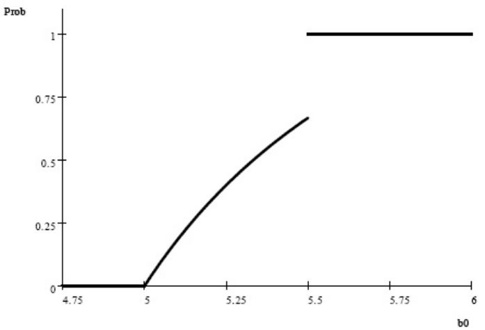
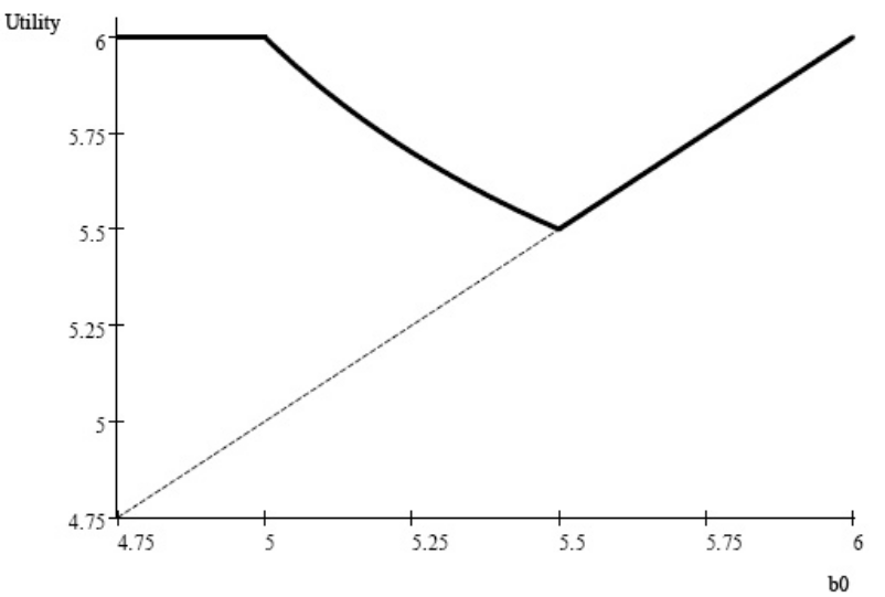
Figure 1(a) summarizes the above equilibrium description by plotting the probability with which the agent recommends project one when $(b_1,b_2)=(1,4)$. Figure 1(b) plots the corresponding ex-ante expected utility for the DM. For , the DM’s expected utility is constant at $𝔼[\max \{b_1,b_2\}]=6$. When $b_0$ increases from $5$ to $5.5$, the DM’s expected utility is strictly decreasing, because the agent’s pandering is exacerbated by a higher outside option value: because of a lack of commitment, a more valuable outside option harms the DM in this region. Finally, when $b_0>5.5$, the DM always chooses the outside option, so her expected utility is just $b_0$.

(a) Probability of recommending project one when $(b_1,b_2)=(1,4)$

(b) Ex-ante expected utility for DM

Figure 1: Pandering in the Binary Example

It is worth noting that if the DM could commit to delegating the project choice to the agent, her expected payoff from delegation would be $𝔼[\max \{b_1,b_2\}]=6$, so she strictly benefits from doing so if and only if $b_0\in (5,6)$. One can also show in this example that if the DM could commit to an arbitrary mechanism without transfers, then for $b_0\in (5,6.6)$, the optimal mechanism can be implemented by asking the agent to recommend a project and committing to exactly the same acceptance vector as in the equilibrium of the game without commitment. In other words, the DM commits to implementing project one whenever it is recommended while only implementing project two with probability $1/4$ when recommended (and implementing the outside option with remaining probability). The difference, however, is that when the DM has committed to this acceptance rule, the agent responds by truthfully recommending the better project rather than pandering. This mechanism gives the DM an expected payoff of $6.6$, which is higher than from full delegation. The DM’s cost of inducing truthful recommendations is the “information rent” she gives the agent by accepting project two sometimes even though she would ex-post prefer not to. When $b_0>6.6$, the optimal mechanism for the DM is to always choose the outside option because it is no longer worth paying the information rent.

In the remainder of the paper, we study a richer model where each project’s value is drawn from a continuous distribution. We show that suitable versions of the above insights continue to apply, and we develop additional insights. Inter alia, we will study general cheap-talk communication from the agent and deal with the issue of multiple equilibria, identify conditions on the projects’ value distributions under which pandering is systematically in the direction of a particular project, perform comparative statics in the outside option and the projects’ value distributions, and show that unlike in this binary example, pandering also generally arises even when the DM can commit to mechanisms without transfers.

3 The Model

3.1 Setup

There are two players: an agent (“he”) and a decision-maker (DM, “she”). The DM must make a choice from the set $\{0,1,\mathrm{\dots },n\}$, where $n\ge 2$. It is convenient to interpret option $0$ as a status quo or outside option for the DM, and $N:=\{1,\mathrm{\dots },n\}$ as a set of alternative projects. Both players enjoy a common payoff if one of the alternative projects is chosen, but this value is private information of the agent. Specifically, each project $i\in N$ yields both players a payoff of $b_i$ that is drawn from a prior distribution $F_i$ and privately observed by the agent. (Throughout, payoffs refer to von Neumann-Morgenstern utilities, and the players are expected utility maximizers.) On the other hand, it is common knowledge that if the outside option is chosen, the agent’s payoff is zero (a normalization), while the DM’s payoff is $b_0>0$.

We maintain the following assumptions on $(F_1,\mathrm{\dots },F_n)$ and $b_0$:

1. For each $i\in N$, $\text{Support}[b_i]=[{\underset{¯}{b}}_i,{\overline{b}}_i]$, with .

2. For each $i\in N$, $F_i$ is absolutely continuous with a density $f_i$ that is strictly positive on $({\underset{¯}{b}}_i,{\overline{b}}_i)$, and .

3. For each pair $i,j\in N$ with $i\ne j$, $\exists \alpha >0$ such that $𝔼[b_i|b_i>\alpha b_j]>b_0$.

4. For any $i,j\in N$, $F_i$ and $F_j$ are independent distributions, but they need not be identical.

After privately observing $𝐛:=(b_1,\mathrm{\dots },b_n)\in ℬ:=\prod _{i=1}^n[{\underset{¯}{b}}_i,{\overline{b}}_i]$, which we also refer to as the agent’s type, the agent sends a cheap-talk or payoff-irrelevant message to the DM, $m\in M$, where $M$ is a large space (e.g. $M={ℝ}_{+}^n$). The DM then chooses a project $i\in N\cup \{0\}$. Aside from the realization of $𝐛$, all aspects of the game are common knowledge. We study (perfect) Bayesian equilibria.

3.2 Discussion of the assumptions

Since both the agent and the DM derive the same payoff, $b_i$, for any $i\in N$, their interests in choosing between the $n$ projects are completely aligned. Assumption (A1) implies that each project has a positive chance of being better for the DM than the outside option; this is without loss of generality because otherwise a project would not be viable. More importantly, (A1) also implies that the agent strictly prefers any project to the outside option, whereas with positive probability, each project is worse than the outside option for the DM. Thus, the conflict of interest is entirely about the outside option: the agent does not internalize the opportunity cost to the DM of implementing a project. What is essential here is that the DM values the outside option more than the agent relative to the alternative projects; allowing for complicates some details of the analysis without adding commensurate insight.

Assumption (A2) is for technical reasons. Assumption (A3) means that the DM’s posterior assessment of any project $i\in N$ becomes more favorable than the outside option if project $i$ is known to be sufficiently better than any other project $j\in N\setminus \{i\}$. Note that given (A1), this is automatically satisfied if ${\underset{¯}{b}}_i>0$ for all $i$. The role of (A3) will be clarified later (see fn. 25), but intuitively, it ensures that if the agent only recommends a project when it is sufficiently better than some other, the DM will wish to implement it.

The independence portion of Assumption (A4) is not essential for our main results, but it makes some of the analysis more transparent. (A4) also allows for non-identical project distributions. Since this is central to our main results, it is worth discussing at some length. Our preferred interpretation is that each project $i$ has some attributes that are publicly observed and some attributes that are privately observed by the agent. For example, if the projects represent academic job candidates, the two components may respectively be a candidate’s vita and the hiring department’s evaluation of her future trajectory. Both aspects can be viewed as initially stochastic, with the distribution $F_i$ capturing the residual uncertainty about $i$’s value after the observable components have been realized and observed by both DM and agent.  Typically, projects will have different realizations of observable information, so that even if projects $i$ and $j$ are initially symmetric, there will be an asymmetry in the residual uncertainty about them, so that $F_i\ne F_j$. One can therefore view the distribution of $b_i$’s as parameterized by some observable information $v_i$, i.e. $F_i(b_i)\equiv F(b_i;v_i)$. The following are two parameterized families of distributions that serve as useful examples:

• Scale-invariant uniform distributions: $b_i$ is uniformly distributed on $[v_i,v_i+\overline{u}]$ for some $\overline{u}>0$ and $v_1\ge v_2\ge \mathrm{\cdots }\ge v_n=0$.

• Exponential distributions: $b_i$ is exponentially distributed on $[0,\mathrm{\infty })$ with mean $v_i$, where $v_1\ge v_2\ge \mathrm{\cdots }\ge v_n>0$.

In certain applications, rather than some attributes being directly observed by the DM, it may be that all aspects are privately observed by the agent, but there are two kinds of information: verifiable or “hard” information, and unverifiable or “soft” information. Under a monotone likelihood ratio condition that is satisfied by the above two families but is considerably more general, analogues of standard “unraveling” arguments (Milgrom, 1981; Seidmann and Winter, 1997) can be used to support an outcome where the agent fully reveals the verifiable attributes. It is then effectively as though the DM directly learns the realizations of these attributes, and again $F_i$ captures the residual soft information about project $i$. Appendix F formalizes this point.

4 Pandering to Persuade

Hereafter, in the main text, we restrict attention to $n=2$, i.e. there are only two alternative projects to the outside option; this substantially simplifies the exposition while conveying all the main insights. We will comment briefly on $n>2$ toward the end of this section but relegate the formal analysis to Appendix D. Given that $n=2$, we use the notation $-i$ to denote project two if $i=1$ and project one if $i=2$.

4.1 Preliminaries

A strategy for the agent is represented by $\mu :ℬ\to \mathrm{\Delta }(M)$, while a strategy for the DM is $\alpha :M\to \mathrm{\Delta }(N\cup \{0\})$, where $\mathrm{\Delta }(\cdot )$ is the set of probability distributions. Since the game is one of cheap talk, the objects of interest are equilibrium mappings from the agent’s type to the DM’s (mixtures over) decisions rather than what messages are used per se. Say that two equilibria are outcome-equivalent if they have the same such mapping for almost all types. A pair of value distributions $(F_1,F_2)$ is said to be generic if $𝔼[b_1]\ne 𝔼[b_2]$ and, moreover, provided that there are at most a countable number of pairs $(x,y)$ such that $x>y>0$ and either $𝔼[b_2|x{b}_1>b_2>y{b}_1]=𝔼[b_1|x{b}_1>b_2>y{b}_1]$ or $𝔼[b_2|b_2>y{b}_1]=𝔼[b_1|b_2>y{b}_1]$.

We begin by establishing a result that substantially simplifies the analysis of equilibria.

Lemma 1.

Fix generic distributions $(F_1,F_2)$ and a generic outside option $b_0$. Then any equilibrium is outcome-equivalent to one in which: (i) the agent plays a pure strategy whose range consists of at most two messages; (ii) the DM’s strategy is such that following any message $m$, if project $i\in N$ is chosen with positive probability then project $-i$ is chosen with zero probability.

The proof of this result and all others not in the text is in Appendix A.

In light of Lemma 1, we focus hereafter on equilibria where the agent chooses a message $i\in N=\{1,2\}$, which is convenient to interpret as the agent recommending project $i$ or ranking project $i$ above $-i$. In turn, the DM’s strategy can now be viewed as a vector of acceptance probabilities, $𝐪:=(q_1,q_2)\in {[0,1]}^2$, where $q_i$ is the probability with which the DM implements project $i$ when the agent recommends project $i$. In other words, if an agent recommends project $i$, a DM who adopts strategy $𝐪$ accepts the recommendation with probability $q_i$ but rejects it in favor of the outside option with probability $1-q_i$.

Given any acceptance vector $𝐪$, the optimal strategy $\mu$ for the agent has

$${\mu }_i(𝐛)=1\text{ if }{q}_i{b}_i>q_{-i}{b}_{-i},$$ (1)

where ${\mu }_i(𝐛)$ denotes the probability with which a type $𝐛$ agent recommends project $i$. Accordingly, in characterizing an equilibrium, we can just focus on the DM’s acceptance vector, $𝐪$, with the understanding that the agent best responds according to (1). For any equilibrium $𝐪$, the optimality of the DM’s strategy combined with (1) implies a pair of conditions for each project $i$:

$q_i>0$ $⟹$ $𝔼\left[b_i\mid q_i{b}_i\ge q_{-i}{b}_{-i}\right]\ge \max \{b_0,𝔼\left[b_{-i}\mid q_i{b}_i\ge q_{-i}{b}_{-i}\right]\},$ (2)

$q_i=1$ $⟸$ $𝔼\left[b_i\mid q_i{b}_i\ge q_{-i}{b}_{-i}\right]>\max \{b_0,𝔼\left[b_{-i}\mid q_i{b}_i\ge q_{-i}{b}_{-i}\right]\}.$ (3)

Condition (2) says that the DM accepts recommendation of project $i$ only if she finds it weakly better than the outside option as well as the other (unrecommended) project, given her posterior which takes the agent’s strategy (1) into consideration. Similarly, (3) says that if she finds the recommended project to be strictly better than both the outside option and the other (unrecommended) project, she must accept that recommendation for sure. These conditions are clearly necessary in any equilibrium; the following result shows that they are also sufficient.

Lemma 2.

If an equilibrium has acceptance vector $𝐪\in {[0,1]}^2$, then (2) and (3) are satisfied for all projects $i$ such that $\mathrm{Pr}\{𝐛:q_i{b}_i\ge q_{-i}{b}_{-i}\}>0$.  Conversely, for any $𝐪\in {[0,1]}^2$ satisfying (2) and (3) for all $i$ such that $\mathrm{Pr}\{𝐛:q_i{b}_i\ge q_{-i}{b}_{-i}\}>0$, there is an equilibrium where the DM plays $𝐪$ and the agent’s strategy satisfies (1).

For expositional convenience, we will focus on equilibria with the property that if a project $i$ has ex-ante probability zero of being implemented on the equilibrium path, then the DM’s acceptance vector has $q_i=0$. This is without loss of generality because there is always an outcome-equivalent equilibrium with this property: if $q_i>0$ but the agent does not recommend $i$ with positive probability, it must be that $q_i{\overline{b}}_i\le q_{-i}{\underset{¯}{b}}_{-i}$, so setting $q_i=0$ does not change the agent’s incentives and remains optimal for the DM with the same beliefs.

We will refer to an equilibrium with $𝐪=\mathrm{𝟎}:=(0,0)$ as a zero equilibrium. If $q_i=1$, we say that the DM rubber-stamps project $i$, since she chooses it with probability one when the agent recommends it. If the DM rubber-stamps both projects, it is optimal for the agent to be truthful in the sense that he always recommends the better project. It is important to emphasize that truthful here is only in the sense of rankings, not in the sense that the agent fully reveals the cardinal values of the projects. Notice that in any non-zero equilibrium, it is optimal for the agent to be truthful if and only if the DM rubber-stamps both projects. Accordingly, we will say that a truthful equilibrium is one where $𝐪=\mathrm{𝟏}:=(1,1)$. An equilibrium is influential if $\min \{q_1,q_2\}>0$, i.e. both projects are implemented on the equilibrium path. We say that the agent panders toward $i$ if $q_i>q_{-i}>0$. The reason is that under this condition, the agent will recommend project $-i$ if it is sufficiently better than $i$, but he distorts his recommendation toward $i$ because he will not recommend $-i$ unless $b_{-i}>\frac{q_i}{q_{-i}}{b}_i$. Note that we do not consider $q_i>0=q_{-i}$ as pandering toward $i$ because in this case the agent can never get project $-i$ implemented. An equilibrium is a pandering equilibrium if there is some $i$ such that the agent panders toward $i$ in the equilibrium. Finally, say that an equilibrium $𝐪$ is larger than another equilibrium ${𝐪}^{\prime }$ if $𝐪>{𝐪}^{\prime }$, and $𝐪$ is better than ${𝐪}^{\prime }$ if $𝐪$ Pareto dominates ${𝐪}^{\prime }$ at the interim stage where the agent has learned his type but the DM has not.

4.2 Main results

The fundamental logic of pandering to persuade is very general because so long as the two projects are not identically distributed, the DM’s beliefs when the agent is truthful will typically favor one project, say project one, over the other. Our goal is to identify when there is a systematic pattern of pandering, namely to understand what attributes of the projects — in terms of their value distributions — cause one project to be pandered toward regardless of the selection of equilibrium and the value of the outside option. Moreover, we would like systematic comparative statics, for instance how the outside option affects the degree of pandering. Such analysis requires an appropriate stochastic ordering of the projects’ value distributions.

Definition 1.

The two projects are strongly ordered if

$𝔼[b_1|b_1>b_2]>𝔼[b_2|b_2>b_1],$ (R1)

and, for any $i\in \{1,2\}$,

$$𝔼[b_i|b_i>\alpha b_{-i}]\text{ is nondecreasing in }\alpha \text{ for }\alpha \in (0,{\overline{b}}_i/{\underset{¯}{b}}_{-i}).$$ (R2)

The first part of the strong ordering condition is mild because when $F_1\ne F_2$, generally $𝔼[b_1|b_1>b_2]\ne 𝔼[b_2|b_2>b_1]$; in this sense, (R1) can be viewed as a labeling convention. Given the labeling, we refer to project one as the conditionally better-looking project because it would generate a higher posterior expectation for the DM if the agent were to truthfully recommend the better project.

Now consider (R2): when $\alpha$ increases, there are two effects on $𝔼[b_i|b_i>\alpha b_{-i}]$. On the one hand, for any given realization of $b_{-i}$, the conditional expectation of $b_i$ increases; call this a conditioning effect. On the other hand, there is a countering selection effect: as $\alpha$ rises, lower realizations of $b_{-i}$ become increasingly likely in the event $\{𝐛:b_i>\alpha b_{-i}\}$. (R2) requires the conditioning effect to at least offset the selection effect. The following lemma provides a useful sufficient condition for this property.

Lemma 3.

Condition (R2) for $i\in \{1,2\}$ is satisfied if $b{f}_{-i}(b)/F_{-i}(b)$ is non-increasing in $b$ for $b\in ({\underset{¯}{b}}_{-i},{\overline{b}}_{-i})$.

Thus, (R2) is assured to hold for $i=1,2$ if the reverse hazard rate of project $-i$, $f_{-i}/F_{-i}$, decreases sufficiently fast. While this is more demanding than log-concavity of $F_j$, Appendix G verifies the sufficient condition for a variety of familiar families of distributions including Pareto distributions, Power function distributions (which subsume uniform distributions), Weibull distributions (which subsume exponential distributions), and Gamma distributions.

Our first main result is:

Theorem 1.

Assume that the projects are strongly ordered.

1. If $𝐪$ is an equilibrium with $q_1>0$, then $q_1\ge q_2$; if in addition , then $q_1>q_2$.

2. There is a largest equilibrium, ${𝐪}^{\ast }$, in the sense that for any other equilibrium $𝐪\ne {𝐪}^{\ast }$, ${𝐪}^{\ast }>𝐪$. Moreover, ${𝐪}^{\ast }$ is the best equilibrium, i.e. it interim Pareto dominates any other equilibrium. There exist $b_0^{\ast }:=𝔼[b_2|b_2>b_1]$ and $b_0^{\ast \ast }\ge b_0^{\ast }$ such that:

   1. If $b_0\le b_0^{\ast }$, then the best equilibrium is the truthful equilibrium, ${𝐪}^{\ast }=(1,1)$.

   2. If $b_0\in (b_0^{\ast },b_0^{\ast \ast }),$ the best equilibrium is a pandering equilibrium, ${𝐪}^{\ast }=(1,q_2^{\ast })$ for some $q_2^{\ast }\in (0,1)$. Moreover, in this region, an increase in $b_0$ strictly increases pandering in the best equilibrium (i.e. $q_2^{\ast }$ strictly decreases) and strictly decreases the interim expected payoffs of both players in the best equilibrium.

   3. If $b_0>b_0^{\ast \ast }$, only the zero equilibrium exists, ${𝐪}^{\ast }=(0,0)$.

Part 1 of the theorem implies that in any equilibrium where project one is recommended on path, either the equilibrium is truthful or there is pandering toward project one, which is conditionally better-looking than project two. Part 2 characterizes the largest equilibrium, which is reasonable to focus on; among other things, it is the best equilibrium. The possible values of the outside option can be partitioned into three distinct regions: when $b_0$ is low, the best equilibrium is truthful; when $b_0$ is intermediate, it is a pandering equilibrium where project one is accepted with probability one whereas project two is accepted with interior probability; and when $b_0$ is large enough, only the zero equilibrium exists. The underlying logic of the pandering equilibrium is similar to that of the example in Section 2, but there is one notable difference in how pandering manifests here. Since the project value distributions are continuous, the agent has an essentially unique best response to any acceptance vector $𝐪>\mathrm{𝟎}$, which is to recommend project one if and only if $q_1{b}_1>q_2{b}_2$. Thus, since $q_1^{\ast }=1$, whenever influential communication is possible, the degree of pandering in the largest equilibrium is measured by how low the acceptance probability of project two is: a lower $q_2^{\ast }$ corresponds to more pandering.

Since $b_0^{\ast }=𝔼[b_2|b_2>b_1]\ge 𝔼[b_2]$, Part 2(a) of Theorem 1 implies that a sufficient condition for existence of a truthful equilibrium is $𝔼[b_2]\ge b_0$, i.e. that the conditionally worse-looking project has higher ex-ante expectation than the outside option. Note that the truthful equilibrium would exist even if , which is possible under strong ordering, as discussed more later. Since $b_0^{\ast \ast }\le 𝔼[b_1|b_1>b_2]$, Part 2(c) of the theorem implies that only the zero equilibrium to exist if $b_0>𝔼[b_1|b_1>b_2]$ (hence, a fortiori, $b_0\ge 𝔼[\max \{b_1,b_2\}]$). Note that this condition is not necessary, however, because even if , only the zero equilibrium will exist if the degree of pandering needed to make project two acceptable to the DM is so high that project one becomes unacceptable when it is recommended. For this reason, $q_2^{\ast }$ is typically bounded away from zero when , and then drops discontinuously to zero when $b_0$ cross the $b_0^{\ast \ast }$ threshold. This is analogous to the discontinuity shown in Figure 1(a) for the agent’s pandering in the example of Section 2.

Part 2(b) of Theorem 1 contains two comparative statics associated with the increase in the value of outside option (in the region where the best equilibrium has pandering). First, as one would expect, an increase in the outside option value leads to a strictly more pandering, because the agent must distort more for the DM to be willing to accept project two when recommended. Less obviously, the DM’s welfare strictly decreases with a higher value of outside option. To see why, note that in a pandering equilibrium, the DM is indifferent between project two and the outside option when the agent recommends the former. This implies that holding fixed the agent’s recommendation strategy, the DM’s utility is the same whether she plays ${𝐪}^{\ast }=(1,q_2^{\ast })$ or just rubber-stamps both projects, $𝐪=(1,1)$. Since in the relevant region a higher $b_0$ induces more pandering, a DM who plays $𝐪=(1,1)$ would be choosing the better project less often when $b_0$ is higher, which implies the welfare result.

When , the value of the outside option is irrelevant for the DM’s welfare since the best equilibrium is truthful. Once $b_0>b_0^{\ast \ast }$, the DM’s welfare is strictly increasing in $b_0$ since the outside option is always chosen. Altogether then, the outside option has a non-monotonic effect on the DM’s expected payoff, just as was seen in Figure 1(b) for the example in Section 2. Naturally, the agent’s welfare is weakly decreasing in $b_0$: it is constant and identical to the DM’s when $b_0\le b_0^{\ast }$, then strictly declines in $b_0$ in the pandering interval $(b_0^{\ast },b_0^{\ast \ast })$, and finally drops to zero once $b_0>b_0^{\ast \ast }$.

The characterization of Theorem 1 provides another interesting insight: when pandering arises, the agent does not benefit from a commitment to truthfully recommend the best alternative. To see this, observe that if the agent were constrained to rank the projects truthfully, the DM would play $𝐪=(1,0)$ when $b_0\in (b_0^{\ast },b_0^{\ast \ast })$. The agent interim — hence, ex-ante — prefers the pandering equilibrium vector $(1,q_2^{\ast })$, since he can still get project one whenever he wants but also chooses to recommend project two if $b_2{q}_2^{\ast }>b_1$. In this sense, cheap-talk about rankings is not self-defeating in the current model: for intermediate conflicts of interest (captured by $b_0$), the agent prefers the equilibrium pandering to tying his hands ex ante to a truthful ranking. Indeed, for any $b_0\in (b_0^{\ast },b_0^{\ast \ast })$, if the DM were to think naively that the agent is always recommending the better project (e.g., because she is not aware of the conflict of interest), the agent would want to change the DM’s beliefs and behavior by convincing the DM that he is in fact pandering (e.g. by making her aware of the conflict of interest).

A related insight is that the alternatives themselves (e.g., recruiting candidates) can also benefit from pandering. This is again because when $b_0\in (b_0^{\ast },b_0^{\ast \ast }),$ project two would never be implemented if the agent ranks projects truthfully while it is implemented with positive probability in the pandering equilibrium. The idea can be illustrated via a faculty hiring application: without pandering, a candidate from a lesser-ranked school would be recommended whenever a committee finds him to be the best, but such a recommendation may never be accepted by the Dean, whose cost of resources is not internalized by the committee. On the other hand, with pandering, the candidate is only recommended when he sufficiently dominates a candidate from a better-ranked school; this happens less often, but the candidate benefits because he is at least approved sometimes when recommended. Moreover, a candidate from a better-ranked school also benefits from pandering because he is recommended more often (even when moderately worse that the other candidate) and is approved when recommended.

The implications of Theorem 1 can be illustrated with explicit formulae for our two leading parametric families of distributions:

Example 1 (Scale-invariant uniform distributions).

Assume that $b_2$ is uniformly distributed on $[0,1],$ while $b_1$ is uniformly distributed on $[v,1+v]$ with $v\in (0,1)$. Strong ordering is satisfied, so Theorem 1 applies. As computed in Appendix C, $b_0^{\ast }=\frac{2+v}{3}$, $q_2^{\ast }=\frac{v}{3b_0-2}$, and $b_0^{\ast \ast }$ is the (unique) solution to $b_0^{\ast \ast }=𝔼[b_1|b_1>(\frac{v}{3b_0^{\ast \ast }-2})b_2]$, which is indeed larger than $b_0^{\ast }$. The degree of pandering increases with $b_0$, i.e. $q_2^{\ast }$ is decreasing in $b_0.$ Moreover, $b_0^{\ast }$ and $q_2^{\ast }$ are increasing in $v$; in this sense, project two becomes more acceptable when project one is stronger.

Example 2 (Exponential distributions).

Assume that $b_1$ and $b_2$ are exponentially distributed with means $v_1$ and $v_2,$ where $v_1>v_2>0$. Strong ordering is satisfied, so Theorem 1 applies. Appendix C computes that $b_0^{\ast }=v_2+\frac{v_1{v}_2}{v_1+v_2}$, $q_2^{\ast }=\frac{v_1}{v_2}\left(\frac{2v_2-b_0}{b_0-v_2}\right)$, and $b_0^{\ast \ast }=\frac{3v_1{v}_2}{v_1+v_2}>b_0^{\ast }$. An increase in $b_0$ leads to more pandering (i.e., $q_2^{\ast }$ falls in $b_0).$ Again, $b_0^{\ast }$ and $q_2^{\ast }$ are increasing in $v$; in this sense, project two becomes more acceptable when project one is stronger. Appendix C also provides a formula for the DM’s expected payoff, which may be useful for applications.

What drives the direction of pandering?

Casual intuition may suggest that the agent will pander toward a project that is ex-ante attractive. Indeed, within the scale-invariant uniform or the exponential family of distributions, our strong ordering condition is equivalent to $v_1>v_2$, and hence agrees with all usual stochastic ordering notions, including likelihood-ratio ordering (and hence with ex-ante expected values).

In general, however, Theorem 1 and condition (R1) reveal that the direction of pandering can be subtle, as it may diverge from what would be suggested by usual stochastic relations. The reason is intimately related to how strategic persuasion works in the current setting. When the agent recommends a project to the DM, he is making a comparative statement about alternative projects by conveying that the project he recommends is better than the other. Thus, what is key for the direction of pandering is the conditional expectation of a project when it is ranked the best. Recall that (R1) says that project one is conditionally better-looking in the sense of having a higher conditional expectation when the agent ranks projects truthfully. Crucially, a project that looks best “in isolation” need not be the one that is conditionally better-looking, because the posterior about the recommended project can depend substantially on the project it is compared against. For this reason, the conditionally better-looking project can be dominated by project two in ex-ante expectation and even in likelihood ratio. The discrete example of Section 2 illustrated this point with respect to ex-ante expectation. More generally, in the current setting of continuous distributions, given any distribution $F_2$ with ${\underset{¯}{b}}_2>0$, there is a family of $F_1$ distributions that are likelihood-ratio dominated by $F_2$ but satisfy (R1).

It is also useful to note that when the agent panders toward project one, he does not necessarily recommend project one more often (i.e. with higher ex-ante probability) than project two; generally, this depends on the projects’ value distributions and the degree of equilibrium pandering. In particular, if project one is suitably weaker than project two when viewed in isolation — e.g. it is first-order stochastically dominated — and pandering is not too severe, then project one will be recommended overall less often, and also selected less often, than project two. This underscores that the pandering distortion is relative to truthful recommendations and occurs when the realization of $b_1$ is lower than but sufficiently close to $b_2$.

The next result further develops the economics of comparative rankings.

Theorem 2.

Fix $b_0$ and an environment $𝐅=(F_1,F_2)$ that satisfies strong ordering. Let $\widetilde{𝐅}=({\tilde{F}}_1,{\tilde{F}}_2)$ be an environment with a weaker slate of alternatives: ${\tilde{F}}_j=F_j$ for some $j$, and for $i\ne j$, either (a) $F_i$ strict likelihood-ratio dominates ${\tilde{F}}_i$ and $\widetilde{𝐅}$ satisfies strong ordering, or (b) ${\tilde{F}}_i$ is a degenerate distribution at zero. Letting ${𝐪}^{\ast }$ and ${\widetilde{𝐪}}^{\ast }$ denote the best equilibria in each of the respective environments, we have ${𝐪}^{\ast }\ge {\widetilde{𝐪}}^{\ast }$. Moreover, ${𝐪}^{\ast }>{\widetilde{𝐪}}^{\ast }$ if ${𝐪}^{\ast }>\mathrm{𝟎}$ and .

Theorem 2 considers two senses in which the slate of alternatives becomes stronger when switching from environment $\widetilde{𝐅}$ to $𝐅$: in case (a), the number of projects is held constant, but the distribution of one project improves in the sense of strict likelihood-ratio dominance; in case (b), the environment $\widetilde{𝐅}$ consists of only one project while the environment $𝐅$ is obtained by adding a new project to $\widetilde{𝐅}$. In either case, the best equilibrium in the stronger environment is at least as large as the original environment, and strictly larger if the original environment did not have a truthful equilibrium and the stronger environment has a non-zero equilibrium. (These caveats are necessary, or else both environments would have the same best equilibrium, either truthful or zero respectively.)

An important implication of Theorem 2 is that the best equilibrium in the stronger environment can be strictly larger if the value distribution that improves is that of project one, even though project one is already accepted with probability one when recommended. In this sense, project two can become more acceptable to the DM when project one becomes stronger, even though project two’s distribution is unchanged. This is entirely due to the property of comparative rankings: an improvement in $F_1$ improves the conditional expectation of project two when it is recommended, holding fixed the equilibrium acceptance vector. Strong ordering then implies the existence of a larger equilibrium if the original equilibrium was not truthful. Examples 1 and 2 illustrate this point: there, a likelihood-ratio improvement of project one corresponds to an increase in $v$ and $v_1$ respectively in the two examples, and as noted there, this causes $b_0^{\ast }$ and $q_2^{\ast }$ to both increase.

Case (b) of Theorem 2 implies that the agent never benefits from “hiding a project.” To fix ideas, suppose the availability of project one is common knowledge between the DM and the agent, but the availability of project two is not. Project two is only available with some probability, and its availability is privately known to the agent. The theorem implies that if the agent can credibly prove the availability of project two, it is always optimal for the agent to do so. It is also possible, for instance, that for each $i$, but $𝔼[b_i|b_i>b_{-i}]>b_0$; in such a case, the agent can get the better project accepted when both are available but neither project accepted if only one of the projects were available.

What if the projects are not strongly ordered?

While strong ordering is essential for delivering the full force — in particular, the comparative statics — of Theorem 1 and Theorem 2, a weaker stochastic ordering suffices to identify a systematic direction of pandering.

Definition 2.

The two projects are weakly ordered if $\forall \alpha \ge 1,𝔼[b_1|b_1>\alpha b_2]>𝔼[b_2|\alpha b_2>b_1]$.

It is straightforward that strong ordering implies weak ordering.  The latter is weaker because it does not require (R2).  Rather, weak ordering allows $𝔼[b_i|b_i>\alpha b_{-i}]$ to decrease in $\alpha$, but requires that the ranking assumed in (R1), i.e. that $𝔼[b_1|b_1>\alpha b_2]>𝔼[b_2|\alpha b_2>b_1]$ when $\alpha =1$, must be preserved for all larger $\alpha$.

Theorem 3.

Assume the two projects are weakly ordered. Then, any influential but non-truthful equilibrium has pandering toward project one.

Proof.

Under weak ordering, there cannot be an equilibrium with $1>q_2=q_1>0$ because then the agent will be truthful, hence $b_0=𝔼[b_1|b_1>b_2]>𝔼[b_2|b_2>b_1]=b_0$, a contradiction. So any non-truthful but influential equilibrium must have either $q_1>q_2>0$ or $q_2>q_1>0$. But the latter configuration cannot be an equilibrium because for $\alpha =\frac{q_2}{q_1}>1$, , hence the DM’s optimality requires $q_1=1$, a contradiction. ∎

This result is tight in the sense that the weak ordering condition is not only sufficient but also almost necessary for pandering to systematically go in the direction of one project. In other words, if projects cannot be weakly ordered (even after relabeling projects), then generally the agent may pander toward either project depending on the outside option. To see this, suppose $𝔼[b_1|b_1>b_2]>𝔼[b_2|b_2>b_1]$ but for some ${\alpha }^{\prime }>1$, . For some $b_0\in (𝔼[b_2|b_2>b_1],𝔼[b_2|b_2>b_1]+\epsilon )$ for a small $\epsilon >0$, there exists a pandering equilibrium $𝐪=(1,q_2)$ with $q_2\in (0,1)$, i.e. the agent panders toward project one. Yet, for some $b_0\in (𝔼[b_1|b_1>{\alpha }^{\prime }{b}_2],𝔼[b_1|b_1>{\alpha }^{\prime }{b}_2]+\epsilon )$ for a small $\epsilon >0$, there is an equilibrium ${𝐪}^{\prime }=(q_1^{\prime },1)$ with $q_1^{\prime }\approx 1/{\alpha }^{\prime }\in (0,1)$, i.e. the agent now panders toward project two.

More than two projects.

Much of the preceding analysis generalizes to $n>2$, as shown formally in Appendix D. The caveats are that for $n>2$, (i) instead of deriving the conclusion of Lemma 1 as a result, we assume the multi-project version of it; (ii) the notion of strong ordering must be appropriately generalized and strengthened; and (iii) the largest equilibrium need not be the best equilibrium for the DM, although it remains so for the agent. Nevertheless, we argue in Appendix D that the largest equilibrium is still compelling to focus on. Subject to these caveats, Theorem 7 in Appendix D generalizes Theorem 1 by establishing that for $n>2$, there are also threshold values, $b_0^{\ast }$ and $b_0^{\ast \ast }$, such that (i) for , there is a truthful equilibrium; (ii) for $b_0\in (b_0^{\ast },b_0^{\ast \ast })$, the largest equilibrium has pandering towards conditionally better-looking projects; and (iii) for $b_0>b_0^{\ast \ast }$, the only equilibrium is the zero equilibrium. Furthermore, Theorem 8 develops an essentially identical analogue to Theorem 2. In particular, these results apply to the scale-invariant and exponential families for $n>2$.

5 Pandering under Commitment

The previous section established that for moderate outside options, pandering necessarily arises in the best cheap-talk equilibrium. An important question is to what extent this is due to the DM’s inability to commit to how she will use any information revealed by the agent. In this section, we study various degrees of commitment power.

5.1 Simple mechanisms

Consider first a simple class of mechanisms where the agent must choose a message $i\in \{1,2\}$, but unlike the cheap-talk game, the DM is now able to commit ex-ante to a vector of acceptance probabilities, $𝐪$, where each $q_i\in [0,1]$. As before, when the agent sends message $i$, the DM chooses project $i$ with probability $q_i$ and the outside option with probability $1-q_i$. We refer to any such mechanism as a simple mechanism. This class of mechanisms can obviously implement any cheap-talk outcome, but also various other outcomes such as full delegation (implemented by setting $𝐪=\mathrm{𝟏}$) and delegation to intermediaries (any ). To see the last point, note that Part 2(b) of Theorem 1 implies that if $b_0$ is such that , then the DM can implement any $𝐪$ such that by delegating decision rights to a third-party who values the outside option at an appropriate $b_0^{\prime }\in (0,b_0)$ and then requiring the third party and the agent to play the cheap-talk game. The presence of such a third party is plausible in a hierarchical organization because often an intermediate boss or a supervisor internalizes the value of the outside option more than the agent but not as much as the principal.

An optimal mechanism within the class of simple mechanisms must solve the following problem:

$$\underset{𝐪\in {[0,1]}^2}{\max }𝔼\left[\sum _{i\in \{1,2\}}{q}_i(b_i-b_0)\cdot {\mathrm{𝟙}}_{\{q_i{b}_i>q_{-i}{b}_{-i}\}}\right]+b_0,$$ (4)

where ${\mathrm{𝟙}}_{\{\cdot \}}$ is an indicator function that equals one in the event of $\{\cdot \}$ and zero otherwise.

In other words, the DM chooses an acceptance vector $𝐪$ knowing that the agent will respond optimally to it in terms of which project he recommends. Note that the DM is allowed to choose a vector $𝐪$ whereby she accepts a recommended project with positive probability even though its posterior value may be strictly less than $b_0$; of course, this requires credible commitment.

It will be useful to introduce a random variable that is the ratio of the project values, $\theta :=\frac{b_1}{b_2}$. The cumulative distributions $F_1$ and $F_2$ induce a cumulative distribution, $F$, over $\theta \in \mathrm{\Theta }:=[\underset{¯}{\theta },\overline{\theta }]$, where $\underset{¯}{\theta }:=\frac{{\underset{¯}{b}}_1}{{\overline{b}}_2}$ and $\overline{\theta }:=\frac{{\overline{b}}_1}{{\underset{¯}{b}}_2}$ if and ${\underset{¯}{b}}_2>0$ and $\overline{\theta }:=\mathrm{\infty }$ otherwise. Let $f$ be the density of $F$. Denoting ${𝐪}^c$ as a solution to (4), we have:

Theorem 4.

Assume the two projects are strongly ordered. Then in any optimal simple mechanism, ${𝐪}^c$, $q_1^c\ge q_2^c$. If the best cheap-talk equilibrium is ${𝐪}^{\ast }=\mathrm{𝟏}$ then the optimal simple mechanism is ${𝐪}^c=\mathrm{𝟏}$. If , then . If $\mathrm{𝟏}>{𝐪}^{\ast }>\mathrm{𝟎}$, then $\mathrm{𝟏}>{𝐪}^c\ge {𝐪}^{\ast }$; moreover, if $f(q_2^{\ast })>0$ then ${𝐪}^c>{𝐪}^{\ast }$.

The first part of the theorem says that in any optimal simple mechanism, the DM accepts project one with a weakly higher probability than project two; hence, if ${𝐪}^c\ne \mathrm{𝟎}$ and the mechanism causes any distortion in the agent’s recommendation, the agent will bias his recommendation toward the conditionally better-looking project. The second part of the theorem says that if cheap talk can sustain truthful rankings, then it cannot be improved on in the class of simple mechanisms. The third part says that if communication cannot be truthful, then the optimal simple mechanism does not fully delegate the project choice to the agent. The last part is the most important: it says that whenever the best cheap-talk equilibrium is influential but has pandering, an optimal simple mechanism also induces the agent to pander, but generally less so than in the cheap-talk game. To see why an optimal mechanism must induce some pandering in this case, assume project two is undesirable if the agent recommends the best project, i.e that . By Theorem 1, this is necessary and sufficient for a truthful equilibrium not to exist in the cheap-talk game. Starting from a commitment to $𝐪=\mathrm{𝟏}$, suppose the DM lowers $q_2$ slightly below 1. The benefit is that when project two is recommended, the outside option $b_0$ will be sometimes realized instead of $b_2$. The cost is that this induces some pandering. However, the benefit is first-order because , while the cost is second-order because there is no pandering distortion at $𝐪=\mathrm{𝟏}$. On balance, reducing $q_2$ slightly below 1 is beneficial.

To see why the optimal mechanism involves reduced pandering relative to communication (so long communication is influential but not truthful), observe that if the DM raises $q_2$ slightly when starting at ${𝐪}^{\ast }$ (with ), there is a first-order benefit of reducing pandering since , but only a second-order cost because $𝔼[b_2|q_2^{\ast }{b}_2>b_1]=b_0$. Extending this logic shows that we must have ${𝐪}^c>{𝐪}^{\ast }$. Since $\mathrm{𝟏}>{𝐪}^c>{𝐪}^{\ast }$, the optimal simple mechanism can be implemented by delegation to an appropriately chosen intermediary, as discussed earlier.

Although Theorem 4 establishes that full delegation (i.e. $𝐪=\mathrm{𝟏}$) is dominated by some other simple mechanism for the relevant outside options, full delegation may be easier to commit to (e.g. through contract, transfer of ownership, eliminating the outside option, etc.). An interesting question then is whether the DM would prefer to delegate or to communicate with the agent if these are the only two choices she has. While delegation eliminates pandering because the agent will always choose the best project, it sometimes leads to a project being implemented even when the DM prefers the outside option. The tradeoff has a simple resolution:

Theorem 5.

Assume the two projects are strongly ordered and that the best cheap-talk equilibrium is ${𝐪}^{\ast }>\mathrm{𝟎}$. Compared to any cheap-talk equilibrium, the DM is ex-ante weakly better off by delegating authority to the agent, and strictly so if .

To see the intuition, suppose . By Theorem 1, the DM is then randomizing between accepting project two and rejecting it when it is recommended, so she must be indifferent between project two and the outside option. Holding the agent’s strategy fixed, the DM’s expected utility is the same whether she plays ${𝐪}^{\ast }$ or always rubber-stamps the agent’s recommendation. Delegation effectively commits the DM to playing the latter strategy and also has the additional benefit of eliminating pandering since the agent will always choose the best project. Therefore, the DM is strictly better off by delegating. Indeed, delegation can be preferred to communication even if ${𝐪}^{\ast }=\mathrm{𝟎}$, so long as .

5.2 General mechanisms

Next we turn to more general mechanisms: can the DM do even better — further mitigate or even eliminate pandering — by using a mechanism that is not simple? For example, could it be optimal to commit to sometimes randomize between both projects, either by themselves or possibly also including the outside option? To answer this question, we solve a full-fledged mechanism design exercise without transfers. By the revelation principle, we can restrict attention to incentive compatible direct revelation mechanisms. It is convenient to view a direct revelation mechanism as a pair of functions $(\overline{x},\overline{y}):\mathrm{\Theta }\times [{\underset{¯}{b}}_2,{\overline{b}}_2]\to A$ where $A:=\{(x,y)\in {[0,1]}^2\mid x+y\le 1\}$. Here, given the ratio $\theta =b_1/b_2$ and the value $b_2$, $\overline{x}(\theta ,b_2)$ is the probability with which project 1 is chosen, $\overline{y}(\theta ,b_2)$ is the probability with which project 2 is chosen, and $1-\overline{x}(\theta ,b_2)-\overline{y}(\theta ,b_2)$ is the probability with which the outside option is chosen.

Lemma 4.

If $(\overline{x},\overline{y})$ is an incentive compatible mechanism, then for all $\theta$, $(\overline{x}(\theta ,b_2),\overline{y}(\theta ,b_2))=(\overline{x}(\theta ,b_2^{\prime }),\overline{y}(\theta ,b_2^{\prime }))$ for any $b_2\ne b_2^{\prime }$.

In words, the above result says that an incentive compatible direct revelation mechanism can only depend on $b_1$ and $b_2$ through the ratio $b_1/b_2$ and not, in addition, on the levels. Importantly, this effectively reduces the two-dimensional type space into a one-dimensional problem. Notice that the utility that type $(\theta ,b_2^{\prime })$ gets from a bundle $(x,y)\in A$ is just a monotone transformation of the utility that type $(\theta ,b_2)$ gets from the same bundle; hence the two types have exactly the same preferences over $A$. However, the DM’s preferences over $A$ are generally not the same for both types of the agent, because the DM cares not only about the ratio $\theta$ but also about how $b_1$ and $b_2$ compare with the outside option, $b_0$. Since any agent type with ratio $\theta$ is indifferent over all bundles in the set $\{(x,y)\in A\mid \theta x+y=C,\text{ for some constant }C\}$, the two types $(\theta ,b_2)$ and $(\theta ,b_2^{\prime })$ would be willing to choose different bundles that lie on the same such indifference curve. The DM may try to exploit this indifference and separate types $(\theta ,b_2^{\prime })$ and $(\theta ,b_2$) when $b_2\ne b_2^{\prime }$. However, Lemma 4 says that this is impossible in an incentive compatible mechanism.

In light of Lemma 4, we can without loss focus on direct revelation mechanisms that map from $\mathrm{\Theta }$ into $A$, i.e. treat the agent’s type as just $\theta$. Since type $\theta$’s preferences over bundles $(x,y)\in A$ can be represented by $u(x,y,\theta ):=x\theta +y$, the problem has a resemblance to standard mechanism design problems with transfers, even though our setting does not have transfers; rather, the probability of choosing project two, $y$, acts like a divisible numeraire. The analogy is imperfect, however, because $y$ is constrained to lie in $[0,1]$ and together with $x$ must further satisfy $x+y\le 1$. This makes the analysis significantly more involved than in standard mechanism design. To proceed, define

$$J(\theta ):=-(1-\theta )b_{0}f(\theta )+{\int }_{\theta }^{\overline{\theta }}\left(𝔼\left[b_2|\frac{b_1}{b_2}=s\right]-b_0\right)f(s)𝑑s.$$ (5)

Intuitively, $J(\cdot )$ is a suitably-constructed “virtual valuation” function. Say that $J(\cdot )$ is piecewise monotone if $\mathrm{\Theta }$ can be partitioned into a finite number of subintervals such that on each subinterval, $J(\cdot )$ is monotone (either nondecreasing or nonincreasing). This is a rather mild regularity condition that permits $J(\cdot )$ to be globally non-monotone.

Theorem 6.

Assume the two projects are strongly ordered and that $J(\cdot )$ is piecewise monotone. If the best cheap-talk equilibrium is , then an optimal simple mechanism is optimal in the class of all mechanisms without transfers.

Hence, under the regularity condition, the insights of Theorem 4 apply in the class of all mechanisms so long as truthful communication cannot be sustained in cheap talk; in particular, an optimal unrestricted mechanism also induces pandering, but to a lesser degree than in cheap talk. Moreover, when the best cheap-talk equilibrium has pandering, the DM cannot do any better than delegating decision-making to an appropriately-chosen intermediary who must then play the cheap-talk game with the agent.

6 Conclusion

This paper has studied strategic communication by an agent who has non-verifiable private information about the benefit of different alternatives and shares a decision maker’s (DM) preferences amongst these. The source of conflict, however, is over an outside option that the DM values but the agent does not fully internalize.

This type of agency problem is salient in many settings that involve some kind of resource allocation. Examples include a seller who vies for a consumer’s purchase, a supplier competing for a firm’s contract, a venture capitalist raising funds from wealthy individuals or institutions, a philanthropist choosing between charities, or a firm allocating its resources between divisions. In each of these cases, the agent typically does not fully internalize the resource cost because he derives private benefits when he sells more, is allocated more resources, manages more money, or is given a larger budget.

The key issue we have focussed on is the nature of cheap-talk communication when the alternatives “look different” to the DM based on either publicly observable attributes or due to verifiable information that has endogenously been revealed by the agent himself. Our core result is that this typically forces pandering in the sense of a systematic distortion in the agent’s recommendations, and hence the DM’s decisions, toward alternatives that are “conditionally better-looking.” Which alternative is conditionally better-looking can be subtle. We have developed comparative statics in the observable information (formally, the value distributions of the alternatives) and in the outside option.

The second part of our analysis focussed on organizational responses to such pandering. If pandering is needed for influential cheap talk, then even a DM with full commitment power would find it optimal to induce pandering from the agent, but to a lesser degree than under cheap talk. Our result about the desirability of full delegation over communication implies that the following simple decision process would improve on pure communication for the DM: request first all verifiable information from the agent (or wait for the publicly observable information to be realized) and then decide between either (i) fully delegating the decision to the agent (with a commitment to not override his choice), and (ii) just going with the outside option. In this organization structure, hard information on the options is all that matters because it determines whether delegation to the agent is warranted or not; cheap talk or soft communication is of no value. This provides a rationale for “no-strings attached” budget allocations, delegation of hiring decisions to subgroups, commitments to buy in buyer-seller relationships, and requirements from venture capitalists or investment funds that investors commit their money for some period of time.

There are many other implications that can be deduced from our analysis. For example, the DM may find it beneficial to reduce or altogether eliminate her outside option, i.e. set $b_0=0$, as this effectively commits her to delegating the project choice to the agent. The DM may be willing to do so even if she must pay to reduce the value of outside option, implying that “burning ships” may be optimal. Alternatively, in some applications it is reasonable to think that the DM is faced with a default of $b_0=0$ and can only improve it at some cost. Suppose that prior to communication, the DM can endogenously choose the value $b_0$ of outside option at a cost $c(b_0)$, where $c(\cdot )$ is strictly increasing. Suppose further that the DM’s choice of $b_0$ is publicly observed prior to the communication game. Then, an application of Theorem 5 shows that the DM should either not invest in the outside option at all (in which case project choice is effectively delegated to the agent) or she makes it so high that it will always be chosen (in which case the agent is irrelevant).

Another set of implications concern the DM’s partial knowledge of projects’ attributes, which is what causes the pandering distortion. Would the DM be better off by not having any (public) information about the projects? This depends on what partial information the DM can observe, because in addition to learning about how the projects compare against each other, the DM may also learn something about how each of them compares with the outside option. Roughly speaking, information that only informs the DM about how the projects compare with one another but not how either compares with the outside option is harmful information that can only create pandering without any countervailing benefit. The DM would prefer to remain ignorant about such information (unless she can commit to ignoring it). Interested readers are referred to Appendix E for a formal development.

The framework we have developed is amenable to a number of extensions that are relevant for applications. We conclude by mentioning a few, again providing details in Appendix E.

An important issue is to allow the DM and the agent to have non-congruent preferences even between the alternatives to the outside option. For instance, a seller may obtain a larger profit margin on certain products, or the head of an organization may have a gender bias or prefer candidates who fit other criteria that the agent does not agree with. A simple way to introduce such conflicts is to assume that the agent derives a benefit $a_i{b}_i$ from project $i$, where $a_i>0$ is common knowledge, while the DM continues to obtain $b_i$ from project $i$. The insights of our basic model carry over to this setting but with some added nuances. For example, simple full delegation becomes less attractive.

Other extensions are particularly relevant for resource allocation problems where a DM decides which projects to provide funding for. These include the DM being privately informed about the opportunity cost of resources; she not only deciding which project to fund, but also how much funding to make available for the project; and/or her being able to fund more than one project if she wishes to. Appendix E shows that our model readily accommodates each of these extensions and that our main themes are robust.

There are a number of more substantial issues that we hope will be studied in future work. Of particular interest is that several agents may compete for resources, in which case each competitor acts like an endogenous outside option for the DM as far as any single agent is concerned. The logic of our analysis suggests that such competition between agents can exacerbate pandering by each agent, and the DM may even be better off by limiting competition.

Appendix A Proofs

Proofs of Lemma 1 and Lemma 2.

See Supplementary Appendix B. ∎

Proof of Lemma 3.

Fix any $i\in \{1,2\}$. For any $y\in (0,{\overline{b}}_i/{\underset{¯}{b}}_{-i})$, we can write

$${\mathrm{{\rm Y}}}_i\left(y\right):=𝔼[b_i|b_i>y{b}_{-i}]={\int }_0^{\mathrm{\infty }}{b}_i{f}_i(b_i|b_i>y{b}_{-i})𝑑b_i={\int }_0^{\mathrm{\infty }}b{\widehat{f}}_i(b;y)𝑑b,$$

where

Condition (R2) states that ${\mathrm{{\rm Y}}}_i(y^{\prime })\ge {\mathrm{{\rm Y}}}_i(y)$ for all ${\overline{b}}_i/{\underset{¯}{b}}_{-i}>y^{\prime }>y>0$. It therefore suffices to show that for any ${\overline{b}}_i/{\underset{¯}{b}}_{-i}>y^{\prime }>y>0$, ${\widehat{f}}_i(\cdot ;y^{\prime })$ dominates ${\widehat{f}}_i(\cdot ;y)$ in likelihood ratio. Since, for any $\tilde{y}\in (0,{\overline{b}}_i/{\underset{¯}{b}}_{-i})$, ${\widehat{f}}_i(\cdot ;\tilde{y})$ has support $[\max \{{\underset{¯}{b}}_i,\tilde{y}{\underset{¯}{b}}_{-i}\},{\overline{b}}_i]$, it is sufficient if

Letting $G(y,b,b^{\prime }):=F_{-i}(\frac{b^{\prime }}{y})/F_{-i}(\frac{b}{y})$ and noting that $G(y,b,b^{\prime })=1$ if $b^{\prime }/y>b/y\ge {\overline{b}}_{-i}$, it follows from the definition of ${\widehat{f}}_i(\cdot ;\cdot )$ that the above sufficient condition is equivalent to

which in turn can be expressed as

(6)

Within the relevant domain, differentiation yields

${\displaystyle \frac{\partial G(y,b,b^{\prime })}{\partial y}}$ $\propto$ $(b/y)F_{-i}(b^{\prime }/y)f_{-i}(b/y)-(b^{\prime }/y)F_{-i}(b/y)f_{-i}(b^{\prime }/y).$

It follows that (6) holds if for any ${\overline{b}}_{-i}\ge b^{\prime }>b\ge {\underset{¯}{b}}_{-i}$, $b\frac{f_{-i}(b)}{F_{-i}(b)}\ge b^{\prime }\frac{f_{-i}(b^{\prime })}{F_{-i}(b^{\prime })}.$ ∎

Proof of Theorem 1.

For any $y>0$, let $\mathrm{\Lambda }(y):=𝔼[b_1|b_1>y{b}_2]-𝔼[b_2|y{b}_2>b_1]$, whenever this is well-defined. Strong ordering implies that $\mathrm{\Lambda }(y)>0$ for any $y\ge 1$ at which it is well-defined.

Step 1: To prove Part 1 of the theorem, pick any equilibrium $𝐪$ with $q_1>0$. Assume, to contradiction, that $q_2>q_1$. Then $𝔼\left[b_1|q_1{b}_1\ge q_2{b}_2\right]=𝔼\left[b_1|b_1\ge \frac{q_2}{q_1}{b}_2\right]>𝔼\left[b_2|\frac{q_2}{q_1}{b}_2\ge b_1\right]=𝔼\left[b_2|q_2{b}_2\ge q_1{b}_1\right]\ge b_0$, where the strict inequality is by strong ordering and that $q_2/q_1\ge 1$, while the weak inequality is because $q_2>0$. But equilibrium now requires that $q_1=1$ (recall condition (3)), a contradiction with $q_2>q_1$. Similarly, if , the same argument applies, except that the contradiction is not with $q_2>q_1$ but rather with .

Part 2 of the theorem is proved in a number of steps. Steps 2–4 below concern the essential properties of the largest equilibrium, ${𝐪}^{\ast }$, and the outside option thresholds, $b_0^{\ast }$ and $b_0^{\ast \ast }$.

Step 2: Plainly, there is a truthful equilibrium ${𝐪}^{\ast }=(1,1)$ when , and this is the largest equilibrium for such $b_0$. Note that for any $b_0>b_0^{\ast }$, there is no equilibrium $𝐪$ with , because in that case the agent always recommends project two, but then , contradicting equilibrium condition (2). By the first part of the theorem, we conclude that for $b_0>b_0^{\ast }$, any non-zero equilibrium $𝐪$ has $q_1>q_2$.

Step 3: Suppose that for all $y>0$, $\mathrm{\Lambda }\left(y\right)>0$. Set . Since $b_0^{\ast }=𝔼[b_2|b_2>b_1]$, it follows that $b_0^{\ast \ast }\ge b_0^{\ast }$, with equality if and only if for all $y\in (0,1)$. Since is continuous in $y$ for all $y>0$, it follows that for any $b_0\in (b_0^{\ast },b_0^{\ast \ast })$, there is some $q_2^{\ast }\in (0,1)$ that solves ; if there are multiple solutions, pick the largest one. Suppose the agent recommends project two if and only if $q_2^{\ast }{b}_2>b_1$. Since , it is optimal for the DM to accept project two with probability $q_2^{\ast }$ when it is recommended. Moreover, , where the last inequality is by the hypothesis that $\mathrm{\Lambda }(y)>0$ for all $y>0$; hence it is also optimal for the DM to accept project one when recommended. Therefore, ${𝐪}^{\ast }=(1,q_2^{\ast })$ is a pandering equilibrium, which by construction is larger than any other equilibrium $𝐪$ with $q_1=1$. Moreover, any non-zero equilibrium $\widetilde{𝐪}$ with has ${\tilde{q}}_1>{\tilde{q}}_2$ (see Step 2), hence there would be a larger equilibrium $𝐪=(1,{\tilde{q}}_2/{\tilde{q}}_1)$, which in turn is weakly smaller than ${𝐪}^{\ast }$. Finally, we don’t need to consider $b_0\ge b_0^{\ast \ast }$ because this violates Assumption (A3).

Step 4: Suppose now that $\mathrm{\Lambda }(y)=0$ for some $y>0$.  Let $\widehat{y}:=\max \{y:\mathrm{\Lambda }(y)=0\}$. Since $\mathrm{\Lambda }(1)>0$, it follows that and $\mathrm{\Lambda }\left(y\right)>0$ for all $y>\widehat{y}$. Set . Plainly, $b_0^{\ast \ast }\ge b_0^{\ast }$, with strict inequality if is strictly decreasing at $y=1$. It follows from the continuity of $𝔼\left[b_2|b_1\le y{b}_2\right]$ in $y$ for $y\in [\widehat{y},1]$ that for all $b_0\in (b_0^{\ast },b_0^{\ast \ast }]$, there is a solution $q_2^{\ast }\in (\widehat{y},1)$ to ; if there are multiple solutions, pick the largest one. By arguments similar to those used in Step 1, $q^{\ast }=(1,q_2^{\ast })$ is a pandering equilibrium that is also the largest among all equilibria. Finally, we must argue that for $b_0>b_0^{\ast \ast }$, the only equilibrium is ${𝐪}^{\ast }=\mathrm{𝟎}$.  Note there is no influential equilibrium by the construction of $b_0^{\ast \ast }$, and by Step 2, any non-influential equilibrium $𝐪$ must have $q_2=0$. But , so there is no equilibrium $𝐪$ with $q_1>0=q_2$.

Step 5: This step shows that ${𝐪}^{\ast }$ is the best equilibrium. Since ${𝐪}^{\ast }=\mathrm{𝟎}$ is the only equilibrium when $b_0>b_0^{\ast \ast }$, assume . Clearly, the agent prefers a larger equilibrium (in the sense that his expected payoff is weakly larger for all $𝐛$ and strictly larger for some $𝐛$), so we need only show that the DM’s welfare is highest at ${𝐪}^{\ast }$.  As shown earlier, implies that the largest equilibrium ${𝐪}^{\ast }$ has $q_1^{\ast }=1$. Suppose there exists another equilibrium .

Consider first $q_1=0$ and $q_2=0$. The DM weakly prefers ${𝐪}^{\ast }$ since she always chooses a project that gives her on expectation at least $b_0$. Consider next $q_1=0$ and $q_2>0$. Then $𝔼[b_2]\ge b_0$, which implies by strong ordering that $𝔼[b_1|b_1\ge b_2]>𝔼[b_2|b_2\ge b_1]\ge 𝔼[b_2]$, hence ${𝐪}^{\ast }=\mathrm{𝟏}$. Clearly, the DM strictly prefers ${𝐪}^{\ast }$ over $𝐪$. Finally, suppose $q_1>0$. Then, by the first part of the theorem, $q_1\ge q_2$. We can assume $q_1=1$, for otherwise there exists another equilibrium ${𝐪}^{\prime }=\frac{1}{q_1}𝐪$ which the DM prefers at least weakly to $𝐪$. Since , it now follows that . Let $\mathrm{\Pi }(\stackrel{~}{}𝐪)$ denote the DM’s expected payoff in an arbitrary equilibrium $\stackrel{~}{}𝐪$. Notice that in computing $\mathrm{\Pi }({𝐪}^{\ast })$ or $\mathrm{\Pi }(𝐪)$, we can keep the agent’s strategy fixed and assume the DM instead adopts both projects with probability one when recommended (even though she may not in equilibrium), because of the DM’s indifference when she adopts project two with strictly interior probability. Thus,

$\mathrm{\Pi }({𝐪}^{\ast })$ $=$

$>$

$=$

where the strict inequality holds because and in this event, $b_2>b_1$ because $q_2^{\ast }\le 1$.

Step 6: Finally, we address the comparative statics when $b_0$ increases within the region $(b_0^{\ast },b_0^{\ast \ast })$. It is clear that $q_2^{\ast }$ strictly decreases in $b_0$ by its construction in Steps 3 and 4. Given this, the same payoff argument as in the final part of Step 4 shows that the DM’s expected payoff strictly decreases in $b_0$.  Plainly, the agent’s interim expected payoff is weakly smaller for all $𝐛$ and strictly so for some $𝐛$ when $b_0$ is larger. ∎

Proof of Theorem 2.

For case (b), where ${\tilde{F}}_i$ is a degenerate distribution at zero, the conclusions of the theorem follow from the observations that if then ${\widetilde{𝐪}}^{\ast }=\mathrm{𝟎}$, and if $𝔼[{\tilde{b}}_j]\ge b_0$ then ${𝐪}^{\ast }=\mathrm{𝟏}$ because $F_j={\tilde{F}}_j$. So assume for the rest of the proof that ${\tilde{F}}_i$ is not degenerate, i.e. case (a) applies. The theorem holds trivially if ${\widetilde{𝐪}}^{\ast }=\mathrm{𝟎}$, so also assume ${\widetilde{𝐪}}^{\ast }>\mathrm{𝟎}$, hence ${\widetilde{𝐪}}^{\ast }=(1,{\tilde{q}}_2^{\ast })\gg \mathrm{𝟎}$. Let $𝐛$ and $\widetilde{𝐛}$ be the random vectors of the project values corresponding to $𝐅$ and $\widetilde{𝐅}$, respectively. First, suppose $i=1$ and ${\underset{¯}{b}}_1\ge {\tilde{q}}_2^{\ast }{\overline{b}}_2$. Then, by strong ordering, it is clear that ${𝐪}^{\ast }>\stackrel{~}{}{𝐪}^{\ast }$: one one just raises the second component of the acceptance vector as high as possible so long as it remains optimal for the DM to accept project two when recommended.

So assume now that either $i=2$ or . Then, we claim that for $m\in \{1,2\}$,

$$𝔼[b_m|{\tilde{q}}_m^{\ast }{b}_m=\underset{k\in \{1,2\}}{\max }{\tilde{q}}_k^{\ast }{b}_k]\ge 𝔼[{\tilde{b}}_m|{\tilde{q}}_m^{\ast }{\tilde{b}}_m=\underset{k\in \{1,2\}}{\max }{\tilde{q}}_k^{\ast }{\tilde{b}}_k].$$ (7)

For $m=i$, inequality (7) follows from the likelihood-ratio dominance hypothesis, since ${\tilde{F}}_j=F_j$. For $m=j$, the argument for inequality (7) is as follows. Define $y:={\tilde{q}}_i^{\ast }/{\tilde{q}}_j^{\ast }$. Then, we can write $𝔼[b_j|{\tilde{q}}_j^{\ast }{b}_j={\max }_{k\in \{1,2\}}{\tilde{q}}_k^{\ast }{b}_k]={\int }_0^{\mathrm{\infty }}b{k}_j(b)𝑑b,$ where $k_j(z):=F_i(\frac{z}{y})f_j(z)/{\int }_0^{\mathrm{\infty }}{F}_i(\frac{\tilde{z}}{y})f_j(\tilde{z})𝑑\tilde{z}$. Likewise, $𝔼[{\tilde{b}}_j|{\tilde{q}}_j^{\ast }{\tilde{b}}_j={\max }_{k\in N}{\tilde{q}}_k^{\ast }{\tilde{b}}_k]={\int }_0^{\mathrm{\infty }}b{\tilde{k}}_j(b)𝑑b$, where ${\tilde{k}}_j(z):={\tilde{F}}_i(\frac{z}{y})f_j(z)/{\int }_0^{\mathrm{\infty }}{\tilde{F}}_i(\frac{\tilde{z}}{y})f_j(\tilde{z})𝑑\tilde{z}$. It suffices to show that the cumulative distribution with density $k_j$ likelihood-ratio dominates that with density ${\tilde{k}}_j$. Note that $k_j$ has support $[\max \{y{\underset{¯}{b}}_i,{\underset{¯}{b}}_j\},{\overline{b}}_j]$, and ${\tilde{k}}_j$ has support $[\max \{y{\underset{¯}{\overset{~}{b}}}_i,{\underset{¯}{b}}_j\},{\overline{b}}_j]$, where ${\underset{¯}{\overset{~}{b}}}_i$ is the infimum of the support of ${\tilde{f}}_i$. Since $F_i$ likelihood-ratio dominates ${\tilde{F}}_i$, ${\underset{¯}{b}}_i\ge {\underset{¯}{\overset{~}{b}}}_i$. Hence, it suffices to show that $\frac{k_j(b^{\prime })}{{\tilde{k}}_j(b^{\prime })}\ge \frac{k_j(b)}{{\tilde{k}}_j(b)}$ for any $b$ and $b^{\prime }$ such that . By the definitions of $k_j$ and ${\tilde{k}}_j$, this is equivalent to showing that $\frac{F_i(z^{\prime })}{{\tilde{F}}_i(z^{\prime })}\ge \frac{F_i(z)}{{\tilde{F}}_i(z)}$ for any $z$ and $z^{\prime }$ such that . But this condition holds if $F_i$ dominates ${\tilde{F}}_i$ in reverse hazard rate, which is indeed the case as $F_i$ likelihood-ratio dominates ${\tilde{F}}_i$.

Given that we have established inequality (7), it now follows that ${𝐪}^{\ast }\ge {\widetilde{𝐪}}^{\ast }$: strong ordering of $𝐅$ combined with (7) for each $m\in \{1,2\}$ implies that there is a weakly larger equilibrium in $𝐅$ than ${\widetilde{𝐪}}^{\ast }$ (one just raises the second component of the acceptance vector as high as possible so long as it remains optimal for the DM to accept project two when recommended).

For the second part of the theorem, assume , for if not the conclusion is trivial. So ${\tilde{q}}_2^{\ast }\in (0,1)$.  The argument used above to prove (7) also reveals that since the likelihood-ratio domination of $F_i$ over ${\tilde{F}}_i$ is strict, $k_j$ strictly likelihood-ratio dominates ${\tilde{k}}_j$, hence the inequality in (7) must hold strictly for $m\in \{1,2\}$. But then $\widetilde{{𝐪}^{\ast }}$ cannot be an equilibrium in environment $𝐅$ because randomization would not be optimal for the DM following a recommendation of project two. It follows from the first part of the theorem that ${𝐪}^{\ast }>{\widetilde{𝐪}}^{\ast }$. ∎

Proof of Theorem 4.

To identify the optimal simple mechanism, it is convenient to use the ratio $\theta :=\frac{b_1}{b_2}$. Recall that $F(\cdot )$ and $f(\cdot )$ are respectively the cdf and density for $\theta \in [\underset{¯}{\theta },\overline{\theta }]$. The DM’s problem is to choose a simple mechanism $(q_1,q_2)\in {[0,1]}^2$ to maximize

$$\mathrm{\Pi }(q_1,q_2)=q_1\left({\int }_{\widehat{\theta }(q_1,q_2)}^{\overline{\theta }}{A}_1(\theta )f(\theta )𝑑\theta \right)+q_2\left({\int }_{\underset{¯}{\theta }}^{\widehat{\theta }(q_1,q_2)}{A}_2(\theta )f(\theta )𝑑\theta \right)+b_0,$$ (8)

where $\widehat{\theta }(q_1,q_2):=q_2/q_1$ while $A_1(\theta ):=𝔼[b_1|b_1/b_2=\theta ]-b_0$ and $A_2(\theta ):=𝔼[b_2|b_1/b_2=\theta ]-b_0$ are the DM’s net benefits from choosing projects 1 and 2, respectively.

We first prove that $q_1\ge q_2$ at any optimum. Suppose to the contrary that . For this to be optimal, the DM should not benefit from raising $q_1$ slightly, or

$0\ge {\displaystyle \frac{\partial \mathrm{\Pi }(q_1,q_2)}{\partial q_1}}$ $={\displaystyle {\int }_{\widehat{\theta }}^{\overline{\theta }}}{A}_1(\theta )f(\theta )𝑑\theta +(\partial \widehat{\theta }/\partial q_1)(q_2{A}_2(\widehat{\theta })-q_1{A}_1(\widehat{\theta }))f(\widehat{\theta })$ (9)

$={\displaystyle {\int }_{\widehat{\theta }}^{\overline{\theta }}}{A}_1(\theta )f(\theta )𝑑\theta +(\partial \widehat{\theta }/\partial q_1)(q_1-q_2)b_{0}f(\widehat{\theta }),$ (10)

where the second equality holds because

$$q_2{A}_2(\widehat{\theta })-q_1{A}_1(\widehat{\theta })=𝔼[q_2{b}_2-q_1{b}_1|b_1/b_2=\widehat{\theta }=q_1/q_2]+(q_1-q_2)b_0=(q_1-q_2)b_0.$$

The second term of (9) is positive since and . This means that . But then

where the two weak inequalities are because of (R2) and $\widehat{\theta }=q_2/q_1>1$, and the strict inequality is by (R1). It follows that $\mathrm{\Pi }(q_1,q_2)$ is maximized at $𝐪=\mathrm{𝟎}$, a contradiction.

Since $q_1\ge q_2$, we can let $q_2=q_1\widehat{\theta }$ for some $\widehat{\theta }\in [0,1]$ and accordingly transform the DM’s problem from (8) to one of choosing $(q_1,\widehat{\theta })\in {[0,1]}^2$ to maximize

$${\mathrm{\Pi }}^{\ast }(q_1,\widehat{\theta }):=\mathrm{\Pi }(q_1,q_1\widehat{\theta })=q_1\left({\int }_{\widehat{\theta }}^{\overline{\theta }}{A}_1(\theta )f(\theta )𝑑\theta +\widehat{\theta }{\int }_{\underset{¯}{\theta }}^{\widehat{\theta }}{A}_2(\theta )f(\theta )𝑑\theta \right)+b_0.$$ (11)

Since this objective function is linear in $q_1$, there is always an optimal solution with either $q_1^c=1$ or $q_1^c=0$ (in the latter case, it immediately follows that $q_2^c=0$); moreover, can be optimal only if the term in parentheses in (11) is nonpositive for all $\widehat{\theta }$.

Differentiate ${\mathrm{\Pi }}^{\ast }(q_1,\widehat{\theta })$ with respect to $\widehat{\theta }$ to obtain

${\displaystyle \frac{\partial {\mathrm{\Pi }}^{\ast }(q_1,\widehat{\theta })}{\partial \widehat{\theta }}}$ $=$ $\left[{\displaystyle {\int }_{\underset{¯}{\theta }}^{\widehat{\theta }}}{A}_2(\theta )f(\theta )𝑑\theta -\left(A_1(\widehat{\theta })-\widehat{\theta }{A}_2(\widehat{\theta })\right)f(\widehat{\theta })\right]q_1$ (12)

$=$ $\left[{\displaystyle {\int }_{\underset{¯}{\theta }}^{\widehat{\theta }}}{A}_2(\theta )f(\theta )𝑑\theta +(1-\widehat{\theta })b_{0}f(\widehat{\theta })\right]q_1,$

where the second equation follows from the observation that for any $\theta$,

$$A_1(\theta )-A_2(\theta )\theta =𝔼[b_1-\theta b_2|b_1/b_2=\theta ]-(1-\theta )b_0=-(1-\theta )b_0.$$ (13)

Suppose first ${𝐪}^{\ast }=\mathrm{𝟏}$. Then, $𝔼[b_1|b_1/b_2\ge 1]>𝔼[b_2|b_1/b_2\le 1]\ge b_0$ (the strict inequality is by (R1)), hence the expression in parentheses in (11) is strictly positive at $\widehat{\theta }=q_2^{\ast }=1$. Therefore any maximizer of (11) has $q_1^c=1$. Further, for any $\widehat{\theta }\le 1$, the second term of (12) is clearly nonnegative; the first term is also nonnegative because

$${\int }_{\underset{¯}{\theta }}^{\widehat{\theta }}{A}_2(\theta )f(\theta )𝑑\theta =F(\widehat{\theta })\left(𝔼[b_2-b_0|b_1\le \widehat{\theta }{b}_2]\right)\ge F(\widehat{\theta })\left(𝔼[b_2-b_0|b_1\le b_2]\right)\ge 0,$$

where the first inequality holds since $𝔼[b_2|b_1\le \widehat{\theta }{b}_2]\ge 𝔼[b_2|b_1\le b_2]$ by (R2) and $\widehat{\theta }\le 1$, and the second inequality holds because $𝔼[b_2|b_1\le b_2]\ge b_0$. Hence, the DM’s objective is nondecreasing in $\widehat{\theta }$. So, if there is some such that $\widehat{\theta }={\widehat{\theta }}^{\ast }$ is optimal, it must be that (12) is zero for all $\widehat{\theta }\in ({\widehat{\theta }}^{\ast },1)$. But this implies that $f(\cdot )=0$ on $({\widehat{\theta }}^{\ast },1)$, which is not possible because the support of $\theta$ is an interval by Assumption (A1). Therefore, the only optimum is $\widehat{\theta }=1$, and consequently ${𝐪}^c=\mathrm{𝟏}$ is the unique optimizer in this case.

Next, assume . To show that , assume, to contradiction, that ${𝐪}^c=1$ is optimal. Then $q_1=1$ and $\widehat{\theta }=1$ maximize (11). Since $\widehat{\theta }=1$, the second term of (12) is zero and the first term is strictly negative because , where the strict inequality is because $F(1)>0$ and (since ). Hence (12) is strictly negative for $\widehat{\theta }=1$ and $q_1=1$, which implies that the value of (11) can be strictly increased by lowering $\widehat{\theta }$, a contradiction.

Finally, assume $\mathrm{𝟏}>{𝐪}^{\ast }>\mathrm{𝟎}$. Then $1=q_1^{\ast }>q_2^{\ast }>0$ by Theorem 1. Since in the best cheap-talk equilibrium, the DM is indifferent between the outside option and project two when the latter is recommended, the DM’s expected payoff in the best cheap-talk equilibrium is the same as it would be if she always adopted a recommended project (keeping fixed the agent’s strategy), which is . It follows that

(14)

where the first inequality is because $q_1^{\ast }>q_2^{\ast }$, and the second inequality is because the DM’s ex-ante utility in a cheap-talk equilibrium cannot be lower than $b_0$. (14) implies that the term in the parentheses of (11) must be strictly positive at an optimum, hence the optimal $q_1=1$. Next, observe that for any , the first term of (12) is nonnegative since

$${\int }_{\underset{¯}{\theta }}^{\widehat{\theta }}{A}_2(\theta )f(\theta )𝑑\theta =F(\widehat{\theta })\left(𝔼[b_2-b_0|b_1\le \widehat{\theta }{b}_2]\right)\ge F(\widehat{\theta })\left(𝔼[b_2-b_0|b_1\le q_2^{\ast }{b}_2]\right)=0,$$

where the final equality is from the DM’s indifference condition for $q_2^{\ast }\in (0,1)$, and the inequality is because $𝔼[b_2|b_1\le \widehat{\theta }{b}_2]\ge 𝔼[b_2|b_1\le q_2^{\ast }{b}_2]$ by strong ordering and $\widehat{\theta }\le q_2^{\ast }$. Moreover, the second term of (12) is nonnegative for all $\widehat{\theta }\le q_2^{\ast }$ and strictly positive if $f(\widehat{\theta })>0$. It follows that no can be optimal, because that would require $f(\cdot )=0$ on some interval strictly within the support. Finally, if $f(q_2^{\ast })>0$, it also follows that the optimal $\widehat{\theta }>q_2^{\ast }$. ∎

Proof of Lemma 4.

See Supplementary Appendix B. ∎

Proof of Theorem 6.

See Supplementary Appendix B. ∎

Proof of Theorem 5.

Assume ${𝐪}^{\ast }>\mathrm{𝟎}$. Theorem 1 (part 2) has established that the DM’s expected utility from any cheap-talk equilibrium $𝐪$ is is no larger than that from ${𝐪}^{\ast }$, so it suffices to show that delegation is weakly preferred to ${𝐪}^{\ast }$, and strictly so if . If ${𝐪}^{\ast }=\mathrm{𝟏}$, then the outcome of delegation is identical to that of ${𝐪}^{\ast }$ and the result is trivially true. For , the result follows from the argument in the proof of Theorem 4 that yielded (14). ∎

The remaining appendices are supplementary and not intended for publication.

Appendix B Omitted Proofs

Proof of Lemma 1.

Here, we will prove part (ii) of the lemma. Part (i) then follows from Lemma 8 in Appendix D. For any $m\in M$, let $\alpha (i|m)$ is the probability that the DM chooses project $i$ following message $m$. As we are interested in outcome-equivalence, we can ignore the behavior of any zero measure set of agent types.

Suppose there is an on-path message $m^{\ast }$ such that $\min \{\alpha \left(1|m^{\ast }\right),\alpha \left(2|m^{\ast }\right)\}>0$. (If $m^{\ast }$ does not exist, we are done.) We can assume that there is some other on-path message that induces a different action distribution from the DM, because otherwise $𝔼\left[b_1\right]=𝔼\left[b_2\right]$, which is non-generic. Moreover, we can assume that no on-path message leads to the outside option with probability 1, since the agent will never (except possibly for a zero measure of types) use such a message given the availability of $m^{\ast }$.

Step 1: There exist constants $q_1>\alpha \left(1|m^{\ast }\right)$ and $q_2>\alpha \left(2|m^{\ast }\right)$ such that for any on-path message $m$, either(i) $\alpha \left(m\right)=\alpha \left(m^{\ast }\right)$, or (ii) $\alpha \left(1|m\right)=0$ and $\alpha \left(2|m\right)=q_2$, or (iii) $\alpha \left(1|m\right)=q_1$ and $\alpha \left(2|m\right)=0$.

To prove this, suppose $m$ is on path and $\alpha \left(m\right)\ne \alpha \left(m^{\ast }\right)$. We cannot have the agent strictly prefer $m^{\ast }$ to $m$ or vice-versa independent of his type, so suppose $\alpha \left(1|m\right)>\alpha \left(1|m^{\ast }\right)$ and $\alpha \left(2|m^{\ast }\right)>\alpha \left(2|m\right)$, with the opposite case treated symmetrically below. Then $m^{\ast }$ will be used by the agent only if

$$b_1\alpha \left(1|m^{\ast }\right)+b_2\alpha \left(2|m^{\ast }\right)\ge b_1\alpha \left(1|m\right)+b_2\alpha \left(2|m\right)\text{,}$$

or $b_2\ge b_{1}k,$ where $k:=\frac{\alpha \left(1|m\right)-\alpha \left(1|m^{\ast }\right)}{\alpha \left(2|m^{\ast }\right)-\alpha \left(2|m\right)}$. If $k\ge 1$, $𝔼\left[b_2|m^{\ast }\right]>𝔼\left[b_1|m^{\ast }\right]$, which cannot be, hence .  Analogously, message $m$ will be used by the agent only if $b_1\ge \frac{b_2}{k}$. Since , , which implies that .

A symmetric argument applies to the case of and , establishing that in this case $\alpha \left(2|m\right)>0=\alpha \left(1|m\right)$.

Finally, note that all on-path messages that lead to (possibly degenerate) randomization between project 1 and the outside option must put the same probability on project 1, call it $q_1$, and this must be strictly larger than $\alpha \left(1|m^{\ast }\right)$ — otherwise they would not be used (except possibly by a zero measure of types). Analogously for project 2 and the outside option.

Step 2: Suppose there is an on-path message $m_1$ such that $\alpha \left(1|m_1\right)=q_1$ and an on-path message $m_2$ such that $\alpha \left(2|m_2\right)=q_2$. We cannot have $q_1=q_2=1$, for then only at most a zero measure of types will induce randomization from the DM. So suppose $q_1=1>q_2$.  Then $m^{\ast }$ will only be used by types such that $b_2>b_1$, contradicting $𝔼\left[b_2|m^{\ast }\right]=𝔼\left[b_1|m^{\ast }\right]$. Similarly for . Therefore, , which implies

$$𝔼\left[b_1|m_1\right]=𝔼\left[b_2|m_2\right]=b_0.$$ (15)

Since $m_1$ is used by the agent when $\frac{q_1-\alpha \left(1|m^{\ast }\right)}{\alpha \left(2|m^{\ast }\right)}{b}_1\ge b_2$, and $m_2$ is used by the agent when$\frac{\alpha \left(1|m^{\ast }\right)}{q_2-\alpha \left(2|m^{\ast }\right)}{b}_1\le b_2$, we can visualize the $b_1-b_2$ rectangle as being partitioned into three regions by the two line segments $b_2=x{b}_1$ and $b_2=y{b}_1$ where $y:=\frac{q_1-\alpha \left(1|m^{\ast }\right)}{\alpha \left(2|m^{\ast }\right)}$ and $x:=\frac{\alpha \left(1|m^{\ast }\right)}{q_2-\alpha \left(2|m^{\ast }\right)}$. Message $m_1$ (or other messages that lead to the same distribution of projects) is used in the bottom region, $m^{\ast }$ (or messages that lead to the same distribution of projects) is used in the middle region, and $m_2$ (or messages that lead to the same distribution of projects) in the top region. By the genericity of the prior distributions, there are at most a countable number of $(x,y)$ that can satisfy $𝔼[b_1|m^{\ast }]=𝔼[b_2|m^{\ast }]$. But then, only non-generic $b_0$ satisfy (15).

Step 3: Suppose that any on-path message $m$ with $\alpha \left(m\right)\ne \alpha \left(m^{\ast }\right)$ has $\alpha \left(2|m\right)=0$.  (A symmetric argument applies to the other case where $\alpha \left(1|m\right)=0$.) Then there is some $m_1$ with $\alpha \left(1|m_1\right)=q_1.$ We must have because otherwise the agent will use $m_1$ whenever $b_1\ge b_2$, contradicting $𝔼\left[b_1|m^{\ast }\right]=𝔼\left[b_2|m^{\ast }\right]$. Thus $𝔼\left[b_1|m_1\right]=b_0$. But now analogously to step 2, we can view the type space as partitioned into two regions by a line segment $b_2=\frac{q_1-\alpha \left(1|m^{\ast }\right)}{\alpha \left(2|m^{\ast }\right)}{b}_1$, with message $m_1$ (or others that lead to the same distribution over projects) being used in the lower cone and $m^{\ast }$ (or other messages that lead to the same distribution over projects) being used in the upper cone. By the genericity of prior distributions, there are most a countable number of values of $y:=\frac{q_1-\alpha \left(1|m^{\ast }\right)}{\alpha \left(2|m^{\ast }\right)}$ that can satisfy $𝔼[b_1|m^{\ast }]=𝔼[b_2|m^{\ast }]$. But then, only non-generic $b_0$ can also satisfy $𝔼[b_1|m_1]=b_0$. ∎

Proof of Lemma 2.

The first statement is immediate. For sufficiency, fix any $𝐪$ satisfying (2) and (3) for all $i$ with $\mathrm{Pr}\{𝐛:q_i{b}_i\ge q_{-i}{b}_{-i}\}>0$. We consider two cases:

(i) Suppose first there is some $i$ with $q_i>0$. Then the agent has a best response, $\mu$, that satisfies (1) and also has the property that any project that is recommended on path has positive ex-ante probability of being recommended. Such a $\mu$ and $𝐪$ are mutual best responses and Bayes Rule is satisfied.  The only issue is assigning an appropriate out-of-equilibrium belief when any off-path project $j$ is recommended; one can specify the off-path belief that $b_k=b_0$ for all $k$, which clearly rationalizes $q_j$.

(ii) Now suppose $q_i=0$ for all $i$. Then for all $i$, $\mathrm{Pr}\{𝐛:q_i{b}_i\ge q_{-i}{b}_{-i}\}=1$ and $𝔼\left[b_i\mid q_i{b}_i\ge q_{-i}{b}_{-i}\right]=𝔼[b_i]$. It follows from (3) that for all $i$, $𝔼[b_i]\le b_0$, and hence there is an equilibrium where the DM always chooses the outside option with “passive beliefs”of maintaining the prior no matter the recommendation, and the agent always recommends project one. ∎

Proof of Lemma 4.

Consider two types $(\theta ,b_2)$ and $(\theta ,b_2^{\prime })$. Then, incentive compatibility means that

$$b_2[\theta \overline{x}(\theta ,b_2)+\overline{y}(\theta ,b_2)]\ge b_2[\theta \overline{x}(\theta ,b_2^{\prime })+\overline{y}(\theta ,b_2^{\prime })]$$

and

$$b_2^{\prime }[\theta \overline{x}(\theta ,b_2)+\overline{y}(\theta ,b_2)]\le b_2^{\prime }[\theta \overline{x}(\theta ,b_2^{\prime })+\overline{y}(\theta ,b_2^{\prime })],$$

implying that $\theta [\overline{x}(\theta ,b_2)+\overline{y}(\theta ,b_2)]=\theta \overline{x}(\theta ,b_2^{\prime })+\overline{y}(\theta ,b_2^{\prime })$. It follows that if $\overline{x}(\theta ,b_2)=\overline{x}(\theta ,b_2^{\prime })$, then $\overline{y}(\theta ,b_2)=\overline{y}(\theta ,b_2^{\prime })$. It thus suffices to show that for every $\theta$, $\overline{x}(\theta ,b_2)=\overline{x}(\theta ,b_2^{\prime })$ for any $b_2,b_2^{\prime }\in [{\underset{¯}{b}}_2,{\overline{b}}_2]$. To prove this, consider a correspondence $X:\mathrm{\Theta }\rightrightarrows [0,1]$ defined by

$$X(\theta )=\{x\in [0,1]\mid \exists b_2\in [{\underset{¯}{b}}_2,{\overline{b}}_2]\text{ s.t. }\overline{x}(\theta ,b_2)=x\}.$$

Pick any selection $\widehat{x}(\cdot )$ from $X(\cdot )$, and for any $\theta$, let $\widehat{y}(\theta )$ be corresponding value of $\overline{y}$, i.e. $\widehat{y}(\theta ):=\overline{y}(\theta ,b_2)$ for any $b_2$ such that $\overline{x}(\theta ,b_2)=\widehat{x}(\theta )$.  For any ${\theta }^{\prime }$ and $\theta$, incentive compatibility implies

$$\theta \widehat{x}(\theta )+\widehat{y}(\theta )\ge \theta \widehat{x}({\theta }^{\prime })+\widehat{y}({\theta }^{\prime })\text{ and }{\theta }^{\prime }\widehat{x}({\theta }^{\prime })+\widehat{y}({\theta }^{\prime })\ge {\theta }^{\prime }\widehat{x}(\theta )+\widehat{y}(\theta ).$$

Rearranging the inequalities yields

$${\theta }^{\prime }[\widehat{x}({\theta }^{\prime })-\widehat{x}(\theta )]\ge \widehat{y}(\theta )-\widehat{y}({\theta }^{\prime })\ge \theta [\widehat{x}({\theta }^{\prime })-\widehat{x}(\theta )].$$

As $\theta \to {\theta }^{\prime }$, it follows that $\widehat{y}(\theta )\to \widehat{y}({\theta }^{\prime })$, which in turn implies that $\widehat{x}(\theta )\to \widehat{x}({\theta }^{\prime })$.

Since the selection $\widehat{x}(\cdot )$ was arbitrary, $X(\cdot )$ must be a single-valued correspondence, which proves the result. ∎

Proof of Theorem 6.

In light of Lemma 4, we can without loss focus on a direct revelation mechanism $(x,y):\mathrm{\Theta }\to A$; in other words, treat the agent’s type as just $\theta$. Let $\mathrm{\Omega }$ be the set of such mappings. Recall the DM’s net benefits from choosing the two projects:

$$A_1(\theta ):=𝔼[b_1|b_1/b_2=\theta ]-b_0,\text{ and }{A}_2(\theta ):=𝔼[b_2|b_1/b_2=\theta ]-b_0.$$

Note that the assumption that the best cheap-talk equilibrium is implies, from Theorem 1, that .

To begin the analysis, assume ; the case of $\overline{\theta }=\mathrm{\infty }$ is treated later. Define the utility of the agent with type $\theta$ when she reports ${\theta }^{\prime }$ as $U({\theta }^{\prime }|\theta ):=\theta x({\theta }^{\prime })+y({\theta }^{\prime })$. Let $u(\theta ):=U(\theta |\theta )$. Notice the resemblance with standard mechanism design with transfers: here, the probability of choosing project 2 serves as a transfer. The analogy is not perfect since $y(\theta )\in [0,1-x(\theta )]$ need to be satisfied. This difference makes the subsequent analysis more involved than in the standard mechanism design exercise.

By the standard argument, incentive compatibility holds if and only if

$$u(\theta )=u(\underset{¯}{\theta })+{\int }_{\underset{¯}{\theta }}^{\theta }x(\tilde{\theta })𝑑\tilde{\theta },$$ (Env)

and

$$x(\cdot )\text{ is nondecreasing.}$$ (M)

Therefore, the DM’s problem is:

$$\underset{(x,y)\in \mathrm{\Omega }}{\max }{\int }_{\underset{¯}{\theta }}^{\overline{\theta }}[A_1(\theta )x(\theta )+A_2(\theta )y(\theta )]f(\theta )𝑑\theta$$ ($P_0$)

subject to $(x,y)\text{ satisfies }(\text{Env})\text{ and }(\text{M}).$

To solve this problem, we first substitute (Env) into the objective function in ($P_0$). Rewrite (Env) as:

$$y(\theta )=-\theta x(\theta )+u(\underset{¯}{\theta })+{\int }_{\underset{¯}{\theta }}^{\theta }x(s)𝑑s.$$ (16)

Substituting (16) into the objective function in ($P_0$) yields:

${\displaystyle {\int }_{\underset{¯}{\theta }}^{\overline{\theta }}}\left[A_1(\theta )x(\theta )-A_2(\theta )\left(\theta x(\theta )-u(\underset{¯}{\theta })-{\displaystyle {\int }_{\underset{¯}{\theta }}^{\theta }}x(s)𝑑s\right)\right]f(\theta )𝑑\theta$ (17)

$=$ $\left({\displaystyle {\int }_{\underset{¯}{\theta }}^{\overline{\theta }}}{A}_2(\theta )f(\theta )𝑑\theta \right)u(\underset{¯}{\theta })+{\displaystyle {\int }_{\underset{¯}{\theta }}^{\overline{\theta }}}\left[\left(A_1(\theta )-A_2(\theta )\theta \right)x(\theta )+A_2(\theta ){\displaystyle {\int }_{\underset{¯}{\theta }}^{\theta }}x(s)𝑑s\right]f(\theta )𝑑\theta$

$=$ $\left({\displaystyle {\int }_{\underset{¯}{\theta }}^{\overline{\theta }}}{A}_2(\theta )f(\theta )𝑑\theta \right)u(\underset{¯}{\theta })+{\displaystyle {\int }_{\underset{¯}{\theta }}^{\overline{\theta }}}\left[-(1-\theta )b_{0}x(\theta )+A_2(\theta ){\displaystyle {\int }_{\underset{¯}{\theta }}^{\theta }}x(s)𝑑s\right]f(\theta )𝑑\theta$

$=$ $\left({\displaystyle {\int }_{\underset{¯}{\theta }}^{\overline{\theta }}}{A}_2(\theta )f(\theta )𝑑\theta \right)u(\underset{¯}{\theta })+{\displaystyle {\int }_{\underset{¯}{\theta }}^{\overline{\theta }}}\left[-(1-\theta )b_{0}f(\theta )+{\displaystyle {\int }_{\theta }^{\overline{\theta }}}{A}_2(s)f(s)𝑑s\right]x(\theta )𝑑\theta ,$

where the second equality follows from (13) and the third equality follows from an application of Fubini’s theorem.

Using the definition of the “virtual valuation” in (5), we can rewrite the objective function in ($P_0$) as

$$𝔼[A_2(\theta )](\underset{¯}{\theta }x(\underset{¯}{\theta })+y(\underset{¯}{\theta }))+{\int }_{\underset{¯}{\theta }}^{\overline{\theta }}J(\theta )x(\theta )𝑑\theta .$$

We now recall the constraint that for all $\theta$, $(x(\theta ),y(\theta ))\in A$, which given $x(\cdot )\in [0,1]$ is equivalent to requiring that for all $\theta$, $y(\theta )\in [0,1-x(\theta )]$. In what follows, we solve a relaxed program by only imposing $y(\cdot )\ge 0$ and $y(\underset{¯}{\theta })\le 1$; we will show that the solution to this relaxed program is such that for all $\theta$, $y(\theta )\in [0,1-x(\theta )]$ and hence solves the original program.

Using (16) and $u(\underset{¯}{\theta })=\underset{¯}{\theta }x(\underset{¯}{\theta })+y(\underset{¯}{\theta })$, the constraint that $y(\cdot )\ge 0$ can be expressed as

$$\forall \theta :-\theta x(\theta )+\underset{¯}{\theta }x(\underset{¯}{\theta })+y(\underset{¯}{\theta })+{\int }_{\underset{¯}{\theta }}^{\theta }x(s)𝑑s\ge 0.$$ (18)

Since (M) implies that the left-hand side of the inequality above is nonincreasing in $\theta$, the constraint will be satisfied for all $\theta$ if it is satisfied at $\theta =\overline{\theta }$. Hence, (18) can be replaced with

$$\overline{\theta }x(\overline{\theta })\le \underset{¯}{\theta }x(\underset{¯}{\theta })+y(\underset{¯}{\theta })+{\int }_{\underset{¯}{\theta }}^{\overline{\theta }}x(s)𝑑s.$$ (19)

Therefore, the original program ($P_0$) can be replaced by the relaxed program

$$\underset{y(\underset{¯}{\theta })\in [0,1],x(\cdot )\in [0,1]}{\max }𝔼[A_2(\theta )](\underset{¯}{\theta }x(\underset{¯}{\theta })+y(\underset{¯}{\theta }))+{\int }_{\underset{¯}{\theta }}^{\overline{\theta }}J(\theta )x(\theta )𝑑\theta$$ ($P_0^{\prime }$)

subject to (M) and (19).

Lemma 5.

In any optimal solution to ($P_{\mathit{0}}^{\mathit{\prime }}$), the constraint (19) binds.

Proof.

Suppose, to contradiction, that there is an optimum at which (19) does not bind. Then (M) and (19) imply that $y(\underset{¯}{\theta })>0$. Since , slightly reducing $y(\underset{¯}{\theta })$ would lead to a strict improvement in the value of the objective in ($P_0^{\prime }$) while still satisfying all the constraints, a contradiction. ∎

Lemma 5 implies that at any optimal solution to ($P_0^{\prime }$),

$$y(\underset{¯}{\theta })=\overline{\theta }x(\overline{\theta })-{\int }_{\underset{¯}{\theta }}^{\overline{\theta }}x(\theta )𝑑\theta -\underset{¯}{\theta }x(\underset{¯}{\theta }),$$ (20)

and hence the program simplifies to:

$$\underset{x(\cdot )\in [0,1]}{\max }𝔼[A_2(\tilde{\theta })]\overline{\theta }x(\overline{\theta })+{\int }_{\underset{¯}{\theta }}^{\overline{\theta }}\left(J(\theta )-𝔼[A_2(\tilde{\theta })]\right)x(\theta )𝑑\theta$$ (P)

subject to (M) and

$$\overline{\theta }x(\overline{\theta })-\underset{¯}{\theta }x(\underset{¯}{\theta })-{\int }_{\underset{¯}{\theta }}^{\overline{\theta }}x(\theta )𝑑\theta \le 1.$$ (21)

Lemma 6.

For some some integer $n>1$, there exist sequences

such that an optimal solution to (P) is given by $\widehat{x}(\cdot )$ is defined as: $\widehat{x}(\underset{¯}{\theta })={\widehat{x}}_1$, and for all $i=1,\mathrm{\dots },n$, $\widehat{x}(\theta )={\widehat{x}}_i$ for $\theta \in ({\widehat{\theta }}_i,{\widehat{\theta }}_{i+1}]$.

Proof.

Existence of an optimal solution to (P) is assured by compactness of the feasible set, so let $x(\cdot )$ be an optimal solution to (P). Since $J(\cdot )$ is piecewise monotone, we can partition $[\underset{¯}{\theta },\overline{\theta }]$ into subintervals ${\{[{\theta }_i,{\theta }_{i+1}]\}}_{i=1,\mathrm{\dots },m}$ for some $m\in \mathbb{N}$, such that $J(\theta )$ is either nondecreasing or nonincreasing within each subinterval. By (M), $x({\theta }_i)\le x({\theta }_{i+1})$. We then construct $\widehat{x}(\cdot )$ for each subinterval $({\theta }_i,{\theta }_{i+1}]$ as follows. There are two cases.

Suppose first $J(\theta )$ is nondecreasing on $[{\theta }_i,{\theta }_{i+1}]$. Then, we set $\widehat{x}(\theta )=x({\theta }_i)$ for $\theta \in ({\theta }_i,{\widehat{\theta }}_i)$ and $\widehat{x}(\theta )=x({\theta }_{i+1})$ for $\theta \in [{\widehat{\theta }}_i,{\theta }_{i+1}]$, for ${\widehat{\theta }}_i\in [{\theta }_i,{\theta }_{i+1}]$ such that and

$${\int }_{{\theta }_i}^{{\theta }_{i+1}}\widehat{x}(\theta )𝑑\theta ={\int }_{{\theta }_i}^{{\theta }_{i+1}}x(\theta )𝑑\theta .$$

Such a ${\widehat{\theta }}_i$ exists because the LHS of the above equation is continuous in ${\widehat{\theta }}_i$, and is no less than then RHS when ${\widehat{\theta }}_i={\theta }_i$ while being no greater than the RHS when ${\widehat{\theta }}_i={\theta }_{i+1}$. (If $i=1$, we also set $\widehat{x}({\theta }_1)={lim}_{\theta \downarrow {\theta }_1}\widehat{x}(\theta )$.) In this case, changing from $x(\cdot )$ to $\widehat{x}(\cdot )$ can only increase the integral term in the objective function of (P) for the subinterval since

${\displaystyle {\int }_{{\theta }_i}^{{\theta }_{i+1}}}\left(J(\theta )-𝔼[A_2(\tilde{\theta })]\right)\widehat{x}(\theta )𝑑\theta -{\displaystyle {\int }_{{\theta }_i}^{{\theta }_{i+1}}}\left(J(\theta )-𝔼[A_2(\tilde{\theta })]\right)x(\theta )𝑑\theta$

$=$ ${\displaystyle {\int }_{{\theta }_i}^{{\theta }_{i+1}}}J(\theta )(\widehat{x}(\theta )-x(\theta ))𝑑\theta \ge {\displaystyle {\int }_{{\theta }_i}^{{\theta }_{i+1}}}J({\widehat{\theta }}_i)(\widehat{x}(\theta )-x(\theta ))𝑑\theta =J({\widehat{\theta }}_i)\left[{\displaystyle {\int }_{{\theta }_i}^{{\theta }_{i+1}}}(\widehat{x}(\theta )-x(\theta ))𝑑\theta \right]=0,$

where the weak inequality follows from the facts that for $\theta \ge {\widehat{\theta }}_i$, $J(\theta )\ge J({\widehat{\theta }}_i)$ and $\widehat{x}(\theta )\ge x(\theta )$, while for , $J(\theta )\le J({\widehat{\theta }}_i)$ and $\widehat{x}(\theta )\le x(\theta )$, and the final equality follows from ${\int }_{{\theta }_i}^{{\theta }_{i+1}}\widehat{x}(s)𝑑s={\int }_{{\theta }_i}^{{\theta }_{i+1}}x(s)𝑑s$. Furthermore, in case $i=m$, the fact that ${\theta }_{i+1}=\overline{\theta }$ and $\widehat{x}({\theta }_{i+1})=x({\theta }_{i+1})$ implies that the first term of the objective function of (P) is unchanged.

Suppose next $J(\theta )$ is nonincreasing on $[{\theta }_i,{\theta }_{i+1}]$. Then, we set $\widehat{x}(\theta )={\check{x}}_i$ for all $\theta \in ({\theta }_i,{\theta }_{i+1}]$, for ${\check{x}}_i\in [x({\theta }_i),x({\theta }_{i+1})]$ such that and

$${\int }_{{\theta }_i}^{{\theta }_{i+1}}\widehat{x}(\theta )𝑑\theta ={\int }_{{\theta }_i}^{{\theta }_{i+1}}x(\theta )𝑑\theta .$$

Clearly, such a ${\check{x}}_i$ exists. (If $i=1$, we also set $\widehat{x}({\theta }_i)={\check{x}}_i$.) Again,changing from $x(\cdot )$ to $\widehat{x}(\cdot )$ can only increase the integral term in the objective function of (P) for the subinterval since, denoting ${\tilde{\theta }}_i:=inf\{\theta \in [{\theta }_i,{\theta }_{i+1}]|x(\theta )\ge \widehat{x}(\theta )={\check{x}}_i\}$,

${\displaystyle {\int }_{{\theta }_i}^{{\theta }_{i+1}}}\left(J(\theta )-𝔼[A_2(\tilde{\theta })]\right)\widehat{x}(\theta )𝑑\theta -{\displaystyle {\int }_{{\theta }_i}^{{\theta }_{i+1}}}\left(J(\theta )-𝔼[A_2(\tilde{\theta })]\right)x(\theta )𝑑\theta$

$=$ ${\displaystyle {\int }_{{\theta }_i}^{{\theta }_{i+1}}}J(\theta )(\widehat{x}(\theta )-x(\theta ))𝑑\theta \ge {\displaystyle {\int }_{{\theta }_i}^{{\theta }_{i+1}}}J({\tilde{\theta }}_i)(\widehat{x}(\theta )-x(\theta ))𝑑\theta =J({\tilde{\theta }}_i)\left[{\displaystyle {\int }_{{\theta }_i}^{{\theta }_{i+1}}}(\widehat{x}(\theta )-x(\theta ))𝑑\theta \right]=0,$

where the weak inequality holds since for $\theta \ge {\tilde{\theta }}_i$, $J(\theta )\le J({\tilde{\theta }}_i)$ and $\widehat{x}(\theta )={\check{x}}_i\le x(\theta )$, while for , $J(\theta )\le J({\tilde{\theta }}_i)$ and $\widehat{x}(\theta )={\check{x}}_i\ge x(\theta )$, and the final equality follows from ${\int }_{{\theta }_i}^{{\theta }_{i+1}}\widehat{x}(s)𝑑s={\int }_{{\theta }_i}^{{\theta }_{i+1}}x(s)𝑑s$. Furthermore, in case $i=m$, the fact that $\widehat{x}({\theta }_{i+1})=\check{x}\le x({\theta }_{i+1})$ implies the first term of the objective function of (P) can have only weakly increased since .

Clearly, the $\widehat{x}(\cdot )$ constructed above for all subintervals is of the form stated in the lemma. Moreover, $\widehat{x}(\cdot )$ satisfies (M) because $x(\cdot )$ satisfies (M) by hypothesis. Further, the facts that $\widehat{x}(\overline{\theta })\le x(\overline{\theta })$, $\widehat{x}(\underset{¯}{\theta })\ge x(\underset{¯}{\theta })$, and ${\int }_{\underset{¯}{\theta }}^{\overline{\theta }}\widehat{x}(\theta )𝑑\theta ={\int }_{\underset{¯}{\theta }}^{\overline{\theta }}x(\theta )𝑑\theta$ imply that $\widehat{x}(\cdot )$ satisfies (21) since $x(\cdot )$ does by hypothesis. As we have shown that $\widehat{x}(\cdot )$ can only increase the value of the objective function, it follows that $\widehat{x}$ is an optimal solution to program (P). ∎

Therefore, we can without loss restrict attention in solving program (P) to step functions that take the form described in Lemma 6. Simplifying both the objective function in (P) and the constraint (21) accordingly, and using the fact that the proof of Lemma 6 bounds the number of steps an optimal solution need take, it follows that there is some integer $N>1$ such that program (P) can be simplified to:

$$\underset{(\widehat{𝒙},\widehat{𝜽})\in A^n,n\in \{2,\mathrm{\dots },N\}}{\max }\sum _{i=1}^{n-1}\left({\int }_{{\widehat{\theta }}_i}^{{\widehat{\theta }}_{i+1}}(J(\theta )-𝔼[A_2(\tilde{\theta })])𝑑\theta \right){\widehat{x}}_i+\left({\widehat{\theta }}_n𝔼[A_2(\tilde{\theta })]+{\int }_{{\widehat{\theta }}_n}^{\overline{\theta }}J(\theta )𝑑\theta \right){\widehat{x}}_n,$$ ($P^{\prime }$)

where for any $n\in \mathbb{N}\setminus \{1\}$,

$A^n:=\{(𝒙,𝜽)\in {[0,1]}^n\times {\mathrm{\Theta }}^n:x_1\le \mathrm{\cdots }\le x_n,\underset{¯}{\theta }={\theta }_1\le \mathrm{\cdots }\le {\theta }_n\le \overline{\theta },{\displaystyle \sum _{i=1}^{n-1}}{\theta }_{i+1}(x_{i+1}-x_i)\le 1\}.$

Lemma 7.

Program ($P^{\mathit{\prime }}$) has a solution in $A^2$.

Proof.

Assume, to contradiction, that there is no solution to the program in $A^2$. Then a solution exists in $A^n$ for some $n>2$ because the feasible set is compact. We first argue that if there is any solution in $A^n$ for some $n>3$, then there is a solution in $A^{n-1}$, which implies by induction that there is a solution in $A^3$. To prove the inductive step, fix a solution to ($P^{\prime }$), $(\widehat{𝒙},\widehat{𝜽})\in A^n$ for some $n>3$.

Case 1: If ${\widehat{x}}_i={\widehat{x}}_{i+1}$ for some or ${\widehat{\theta }}_i={\widehat{\theta }}_{i+1}$ for some $1\le i\le n$, then there is clearly an equivalent solution in $A^{n-1}$.

Case 2: If Case 1 does not apply, then $\widehat{𝒙}$ and $\widehat{𝜽}$ are strictly increasing sequences. We can then change ${\widehat{x}}_{n-1}$ and ${\widehat{x}}_{n-2}$ in opposite directions (raising one and lowering the other) while keeping ${\sum }_{i=1}^{n-1}{\widehat{\theta }}_{i+1}({\widehat{x}}_{i+1}-{\widehat{x}}_i)$ constant and hence staying within $A^n$ (note that $n>3$ ensures that $x_{n-2}$ can be lowered). Since the objective function in ($P^{\prime }$) is linear in each ${\widehat{x}}_i$, it must be one of these two kinds of changes does not affect the value of the objective function. One can then continue making the change until either ${\widehat{x}}_{n-1}={\widehat{x}}_n$ or ${\widehat{x}}_{n-1}={\widehat{x}}_{n-2}$ or ${\widehat{x}}_{n-2}={\widehat{x}}_{n-3}$ binds, at which point Case 1 applies.

Therefore, we conclude that there is a solution to ($P^{\prime }$), $(\widehat{𝒙},𝜽)\in A^3$. Since by hypothesis there is no solution in $A^2$, it must be that , for otherwise the solution can be redefined to be in $A^2$ just as Case 1 above. Furthermore, we must have , because an argument akin to the one used in Case 2 above shows that otherwise there would be an equivalent solution in $A^2$. This implies that , for otherwise it would remain optimal to raise ${\widehat{x}}_2$ until it coincides with ${\widehat{x}}_3$ (this is feasible because raising ${\widehat{x}}_2$ only relaxes the last requirement in the definition of $A^3$), which cannot be. But then reducing ${\widehat{x}}_2$ would strictly improve the value of the objective function, so it must be that this is not feasible in $A^3$, which implies that $1={\widehat{\theta }}_3-({\widehat{\theta }}_3-{\widehat{\theta }}_2){\widehat{x}}_2$, and consequently ${\widehat{\theta }}_3>1$.

The derivative of the objective function in ($P^{\prime }$) with respect to ${\widehat{\theta }}_3$ is

$\left(𝔼[A_2(\tilde{\theta })]-J({\widehat{\theta }}_3)\right)(1-{\widehat{x}}_2)$ $=$ $\left[{\displaystyle {\int }_{\underset{¯}{\theta }}^{\overline{\theta }}}{A}_2(s)f(s)𝑑s+(1-{\widehat{\theta }}_3)b_{0}f({\widehat{\theta }}_3)-{\displaystyle {\int }_{{\widehat{\theta }}_3}^{\overline{\theta }}}{A}_2(s)f(s)𝑑s\right](1-{\widehat{x}}_2)$

$=$

where the first equality is from definitions, and the inequality holds because ${\widehat{x}}_2\in (0,1)$ and

which in turn is because of strong ordering, ${\widehat{\theta }}_3>1$, and since .

It follows that lowering ${\widehat{\theta }}_3$ slightly strictly improves the value of the objective function, and this is feasible because lowering ${\widehat{\theta }}_3$ slightly only relaxes the last requirement in the definition of $A^3$. But this contradicts $(\widehat{𝒙},𝜽)\in A^3$ being optimal. ∎

By Lemma 7, we can simplify program ($P^{\prime }$) to:

$$\underset{({\widehat{x}}_1,{\widehat{x}}_2,\widehat{\theta })\in A^{\prime }}{\max }\left({\int }_{\underset{¯}{\theta }}^{\widehat{\theta }}(J(\theta )-𝔼[A_2(\tilde{\theta })])𝑑\theta \right){\widehat{x}}_1+\left(\widehat{\theta }𝔼[A_2(\tilde{\theta })]+{\int }_{\widehat{\theta }}^{\overline{\theta }}J(\theta )𝑑\theta \right){\widehat{x}}_2,$$ ($P^{\prime \prime }$)

where

$$A^{\prime }:=\{({\widehat{x}}_1,{\widehat{x}}_2,\widehat{\theta })|0\le {\widehat{x}}_1\le {\widehat{x}}_2\le 1;\widehat{\theta }\in [\underset{¯}{\theta },\overline{\theta }];\widehat{\theta }({\widehat{x}}_2-{\widehat{x}}_1)\le 1\}.$$

We will argue that any solution to ($P^{\prime \prime }$) also solves the original program ($P_0$) and can be implemented by a simple mechanism. There are three possibilities to consider.

First, suppose that a solution to ($P^{\prime \prime }$) has ${\widehat{x}}_1>0$. Then ${\widehat{x}}_2>0$ and moreover the coefficient of ${\widehat{x}}_1$ in ($P^{\prime \prime }$) must be nonnegative, or else one could strictly improve the objective by lowering ${\widehat{x}}_1$ while keeping ${\widehat{x}}_2$ and $\widehat{\theta }$ unchanged. Since the coefficient of ${\widehat{x}}_1$ in ($P^{\prime \prime }$) is nonnegative, an optimum is also obtained by keeping the same ${\widehat{x}}_2$ and $\widehat{\theta }$ but setting ${\widehat{x}}_1={\widehat{x}}_2$. Then, by (20), $y(\underset{¯}{\theta })=0$. This solves the original program ($P_0$) because the outcome can implemented by a feasible mechanism $(x,y)$ where for all $\theta$, $x(\theta )={\widehat{x}}_2$ and $y(\theta )=0$; note that this obviously satisfies the feasibility constraint that $y(\theta )\le 1-x(\theta )$ for all $\theta$. In turn, this optimal mechanism can be implemented by a simple mechanism with $𝐪=({\widehat{x}}_2,0)$.

Next, suppose that that ${\widehat{x}}_2={\widehat{x}}_1=0$ at a solution to ($P^{\prime \prime }$). Then by (20), $y(\underset{¯}{\theta })=0$. This outcome can be implemented by a feasible mechanism $(x,y)$ where $x(\theta )=0$ and $y(\theta )=0$ for all $\theta$. Note that obviously satisfies the feasibility constraint $y(\theta )\le 1-x(\theta )$ for all $\theta$. Since the DM always picks the outside option at this optimal mechanism, it can be implemented by a simple mechanism with $𝐪=\mathrm{𝟎}$.

Finally, suppose ${\widehat{x}}_2>0={\widehat{x}}_1$ at a solution to ($P^{\prime \prime }$). It must be that the coefficient of ${\widehat{x}}_2$ in ($P^{\prime \prime }$) is nonnegative, or else one could strictly improve the objective by lowering ${\widehat{x}}_2$ while keeping ${\widehat{x}}_1$ and $\widehat{\theta }$ unchanged. Therefore, it is also optimal to set ${\widehat{x}}_2=\min \{1,1/\widehat{\theta }\}$. This solution can be implemented by a feasible mechanism $(x,y)$, where $x(\theta )=0$ for and $x(\theta )=\min \{1,1/\widehat{\theta }\}$ for $\theta >\widehat{\theta }$, and $y(\theta )=\min \{\widehat{\theta },1\}$ for and $y(\theta )=0$ for $\theta >\widehat{\theta }$; since this satisfies both (20) and the feasibility constraint that $y(\theta )\in [0,1-x(\theta )]$ for all $\theta$, it also solves the original program ($P_0$). In turn, this optimal mechanism can be implemented by a simple mechanism with $𝐪=(\min \{1,\frac{1}{\widehat{\theta }}\},\min \{\widehat{\theta },1\})$. Notice in this simple mechanism the agent will recommend project two if and project one if $b_1/b_2>\widehat{\theta }$. In the former case, project two is implemented with probability $\min \{\widehat{\theta },1\}$ and the outside option with complementary probability; in the latter case, project one is implemented with probability $\min \{1,1/\widehat{\theta }\}$ while the outside option is implemented with complementary probability.

Summarizing, we have shown that the optimal mechanism is implemented by a simple mechanism. This completes the proof under the assumption that .

The case of $\overline{\theta }=\mathrm{\infty }$.

Hereafter assume $\overline{\theta }=\mathrm{\infty }$. This introduces two difficulties with the method used above for : first, the application of Fubini’s theorem to derive (17) is not necessarily valid since it is possible that $𝔼[\theta ]=\mathrm{\infty }$; second, objects such as $x(\overline{\theta })$ and hence constraints such as (19) are not well defined. We thus take a different approach. Note that the value of ($P_0$) is bounded because for $i=1,2$.

To begin, consider a subproblem $[P_t]$ in which the agent draws $\theta$ from $[\underset{¯}{\theta },t]$ for , according to density $g_t(\theta ):=f(\theta )/F(t)$. Analogous to ($P_0$), the DM’s objective is to now maximize

$${\mathrm{\Phi }}_t(x,y):=\frac{1}{F(t)}{\int }_{\underset{¯}{\theta }}^t[x(\theta )A_1(\theta )+y(\theta )A_2(\theta )]f(\theta )𝑑\theta .$$

The associated virtual value is given by

$$J_t(\theta ):=-(1-\theta )g_t(\theta )+{\int }_{\theta }^t{A}_2(s)g_t(s)𝑑s=\frac{J(\theta )}{F(t)}-\frac{{\int }_t^{\mathrm{\infty }}{A}_2(s)f(s)𝑑s}{F(t)}.$$

It follows from our preceding analysis that there is a simple mechanism that is optimal in this subproblem. In particular, by Theorem 4, there exists an optimal simple mechanism indexed by $(\widehat{\theta },\overline{x})\in {[0,1]}^2$ such that $(x(\theta ),y(\theta ))=(0,\widehat{\theta }\overline{x})$ for , and $(x(\theta ),y(\theta ))=(\overline{x},0)$ for $\theta \in (\widehat{\theta },t]$.

There exists a sequence ${\{t_n\}}_{n=1}^{\mathrm{\infty }}$ with $t_n\to \mathrm{\infty }$ as $n\to \mathrm{\infty }$ such that for each $n$ the simple mechanism $(x_{t_n},y_{t_n})$ indexed by $({\widehat{\theta }}_{t_n},{\overline{x}}_{t_n})\in {[0,1]}^2$ is optimal for subproblem $[P_{t_n}]$. As $n\to \mathrm{\infty }$, $(x_{t_n},y_{t_n})$ converges (in subsequence) to a simple mechanism $(x^{\ast \ast },y^{\ast \ast })$ indexed by $({\widehat{\theta }}^{\ast \ast },{\overline{x}}^{\ast \ast })={lim}_{n\to \mathrm{\infty }}({\widehat{\theta }}_{t_n},{\overline{x}}_{t_n})$.

Fix any feasible mechanism $(x,y):[\underset{¯}{\theta },\mathrm{\infty })\to A$ for the original problem. Its restriction to $[\underset{¯}{\theta },t_n]$, is clearly feasible for the subproblem $[P_{t_n}]$. Since $(x_{t_n},y_{t_n})$ is optimal for subproblem $[P_{t_n}]$, we have that for each $n$,

$${\mathrm{\Phi }}_{t_n}(x_{t_n},y_{t_n})\ge {\mathrm{\Phi }}_{t_n}(x^{t_n},y^{t_n}).$$ (22)

As $n\to \mathrm{\infty }$, the right side of (22) converges to

$$\underset{n\to \mathrm{\infty }}{lim}{\mathrm{\Phi }}_{t_n}(x^{t_n},y^{t_n})=\underset{n\to \mathrm{\infty }}{lim}{\mathrm{\Phi }}_{t_n}(x,y)={\int }_{\underset{¯}{\theta }}^{\mathrm{\infty }}[x(\theta )A_1(\theta )+y(\theta )A_2(\theta )]f(\theta )𝑑\theta ,$$

which is the value of the original objective function ($P_0$) under $(x,y)$.

Meanwhile, as $n\to \mathrm{\infty }$, the left side of (22) converges to

$\underset{n\to \mathrm{\infty }}{lim}{\mathrm{\Phi }}_{t_n}(x_{t_n},y_{t_n})$ $=\underset{n\to \mathrm{\infty }}{lim}{\displaystyle \frac{{\overline{x}}_{t_n}}{F(t_n)}}\left({\displaystyle {\int }_{\underset{¯}{\theta }}^{{\widehat{\theta }}_{t_n}}}{A}_1(\theta )f(\theta )𝑑\theta +{\widehat{\theta }}_{t_n}{\displaystyle {\int }_{{\widehat{\theta }}_{t_n}}^{t_n}}{A}_2(\theta )f(\theta )𝑑\theta \right)$

$={\overline{x}}^{\ast \ast }\left({\displaystyle {\int }_{\underset{¯}{\theta }}^{{\widehat{\theta }}^{\ast \ast }}}{A}_1(\theta )f(\theta )𝑑\theta +{\widehat{\theta }}^{\ast \ast }{\displaystyle {\int }_{{\widehat{\theta }}^{\ast \ast }}^{\mathrm{\infty }}}{A}_2(\theta )f(\theta )𝑑\theta \right)$

$={\displaystyle {\int }_{\underset{¯}{\theta }}^{\mathrm{\infty }}}[x^{\ast \ast }(\theta )A_1(\theta )+y^{\ast \ast }(\theta )A_2(\theta )]f(\theta )𝑑\theta ,$

which is the value of the original objective function ($P_0$) under $(x^{\ast \ast },y^{\ast \ast })$.

Since the inequality in (22) is preserved in the limit as $n\to \mathrm{\infty }$, the simple mechanism $(x^{\ast \ast },y^{\ast \ast })$ gives a weakly higher value than $(x,y)$ in the original problem ($P_0$). Since $(x,y)$ is an arbitrary feasible mechanism, $(x^{\ast \ast },y^{\ast \ast })$ is optimal in the original problem, thus establishing the optimality of a simple mechanism. ∎

Appendix C Leading Examples

This Appendix provides detailed computations for the leading examples with $n=2$. We prove that they satisfy strong ordering and verify the expressions provided in Example 1 and Example 2.

C.1 Scale-invariant uniform distributions

Assume that $b_2$ is uniformly distributed on $[0,1],$ while $b_1$ is uniformly distributed on $[v,1+v]$ with $v\in (0,1)$. Assumption (A1) requires ; this also guarantees (A3).

Strong ordering: We compute

$$𝔼[b_2|b_2>\alpha b_1]=\frac{{\int }_v^{1+v}{\int }_{\alpha b_1}^1{b}_2𝑑b_2𝑑b_1}{{\int }_v^{1+v}{\int }_{\alpha b_1}^1𝑑b_2𝑑b_1}=\frac{3v^2{\alpha }^2+3v{\alpha }^2+{\alpha }^2-3}{3\alpha +6v\alpha -6}\text{ for }\alpha \in [0,\frac{1}{1+v}],$$

and

$$𝔼[b_2|b_2>\alpha b_1]=\frac{{\int }_v^{1/\alpha }{\int }_{\alpha b_1}^1{b}_2𝑑b_2𝑑b_1}{{\int }_v^{1/\alpha }{\int }_{\alpha b_1}^{1}1𝑑b_2𝑑b_1}=\frac{2}{3}+\frac{\alpha }{3}v\text{ for }\alpha \in (\frac{1}{1+v},\frac{1}{v}].$$ (23)

Both expressions are increasing in $\alpha$ in the relevant range.  Note that $𝔼[b_2|b_2>\alpha b_1]$ is not defined for $\alpha >1/v$.

Similarly, it can be computed that

(27)

which is nondecreasing in $\alpha$.

Therefore, (R2) is satisfied. It is also routine to verify that (R1) is satisfied using formulas (23) and (27) with $\alpha =1$. We conclude that strong ordering holds.

The Largest Equilibrium: From Theorem 1 and formula (23),

$$b_0^{\ast }=𝔼[b_2|b_2>b_1]=\frac{2}{3}+\frac{v}{3}.$$

For $b_0>b_0^{\ast }$, a pandering equilibrium ${𝐪}^{\ast }=(1,q_2^{\ast })$ with $q_2^{\ast }\in (0,1)$ requires $𝔼[b_2|b_2>b_1/q_2^{\ast }]=b_0$. Substituting from (23) yields the solution

$$q_2^{\ast }(b_0)=\frac{v}{3b_0-2}$$ (28)

so long as the right hand side above is larger than $v$, which is guaranteed since . That $q_1^{\ast }=1$ implies $𝔼[b_1|b_1>q_2^{\ast }(b_0)b_2]\ge b_0$, into which we substitute (28) to obtain

$$𝔼\left[b_1|b_1>\frac{v}{3b_0-2}{b}_2\right]\ge b_0.$$

By substituting from (27), it can be verified that the left-hand side of the above expression is continuous and weakly decreasing in $b_0$, while the right-hand side is, obviously, strictly increasing. Moreover, by the definition of $b_0^{\ast }$, $𝔼\left[b_1|b_1>\frac{v}{3b_0^{\ast }-2}{b}_2\right]=𝔼[b_1|b_1>b_2]>b_0^{\ast }$. Therefore, there is a unique $b_0^{\ast \ast }$ such that

$$𝔼\left[b_1|b_1>\frac{v}{3b_0^{\ast \ast }-2}{b}_2\right]=b_0^{\ast \ast },$$

and $b_0^{\ast \ast }>b_0^{\ast }$. It can be verified that if and only if . It follows that a pandering equilibrium ${𝐪}^{\ast }=(1,q_2^{\ast })$ with $q_2^{\ast }\in (0,1)$ exists if and only if $b_0\in (b_0^{\ast },\min \{1,b_0^{\ast \ast }\}).$ If (i.e., , then for $b_0\in (b^{\ast \ast },1)$ the only equilibrium is $𝐪=(0,0)$.

Remark 1.

Finally, what happens if $b_0>1$, so that Assumptions (A1) and (A3) fail? If , then , hence $𝐪=(0,0)$ is the only equilibrium. If $v>\frac{1}{2},$ then for $b_0\in (1,\frac{1}{2}+v),$ $𝐪=(1,0)$ is the only equilibrium, whereas for $b_0>\frac{1}{2}+v$, $𝐪=(0,0)$ is the only equilibrium. Thus, a violation of (A1) and (A3) allow for the non-influential equilibrium $(1,0)$ to be the largest equilibrium for certain values of $b_0$.

C.2 Exponential distributions

Assume that $b_1$ and $b_2$ are exponentially distributed with respective means $v_1$ and $v_2$, where $v_1>v_2>0$. Assumption (A1) is obviously satisfied for any $b_0\in {ℝ}_{++}$; we will show below that (A3) requires .

Strong Ordering: Denoting the project densities respectively by $f_1(\cdot )$ and $f_2(\cdot ),$ we have that

$𝔼[b_1|b_1>b_2]$ $=$ ${\displaystyle \frac{{\int }_0^{\mathrm{\infty }}(𝔼[b_1>b_2|b_2]\mathrm{Pr}(b_1>b_2|b_2)f_2(b_2)d{b}_2}{{\int }_0^{\mathrm{\infty }}\mathrm{Pr}(b_1>b_2|b_2)f_2(b_2)𝑑b_2}}$

$=$ ${\displaystyle \frac{v_1+v_2}{v_1}}{\displaystyle {\int }_0^{\mathrm{\infty }}}(v_1+b_2)e^{-\frac{1}{v_1}{b}_2}\left({\displaystyle \frac{1}{v_2}}{e}^{-\frac{1}{v_2}{b}_2}\right)𝑑b_2$

$=$ ${\displaystyle {\int }_0^{\mathrm{\infty }}}(v_1+b_2)\left({\displaystyle \frac{v_1+v_2}{v_1{v}_2}}\right)e^{-\left(\frac{v_1+v_2}{v_1{v}_2}\right)b_2}𝑑b_2$

$=$ $v_1+{\displaystyle \frac{v_1{v}_2}{v_1+v_2}}.$

Similarly,

$$𝔼[b_2|b_2>b_1]=v_2+\frac{v_1{v}_2}{v_1+v_2}.$$

Plainly, (R1) is satisfied. Moreover, since $\alpha b_i$ is exponentially distributed with mean $\alpha v_i$, the above calculations imply

$$𝔼[b_i|b_i>\alpha b_j]=v_i+\frac{\alpha v_i{v}_j}{v_i+\alpha v_j}.$$ (29)

Since the right-hand side above is strictly increasing in $\alpha$ for any $\alpha \in {ℝ}_{+}$, (R2) is satisfied and hence strong ordering holds. Note that since ${lim}_{\alpha \to \mathrm{\infty }}𝔼[b_i|b_i>\alpha b_j]=2v_i,$ Assumption (A3) requires

The Largest Equilibrium: From Theorem 1 and equation (29),

$$b_0^{\ast }=𝔼[b_2|b_2>b_1]=v_2+\frac{v_1{v}_2}{v_1+v_2}.$$

For $b_0>b_0^{\ast }$, a pandering equilibrium $𝐪=(1,q_2^{\ast })$ with $q_2^{\ast }\in (0,1)$ requires $𝔼[b_2|b_2>b_1/q_2^{\ast }]=b_0$. Substituting from (29) yields the solution

$q_2^{\ast }(b_0)={\displaystyle \frac{v_1}{v_2}}\left({\displaystyle \frac{2v_2-b_0}{b_0-v_2}}\right).$ (30)

That $q_1^{\ast }=1$ implies $𝔼[b_1|b_1>q_2^{\ast }(b_0)b_2]\ge b_0$, into which we substitute (29) to obtain

$3v_1-b_0{\displaystyle \frac{v_1}{v_2}}\ge b_0.$

Since the left-hand side of the this inequality is decreasing in $b_0$ and the right-hand side is increasing in $b_0,$ the inequality is satisfied if and only if

$$b_0\le b_0^{\ast \ast }=\frac{3v_1{v}_2}{v_2+v_1}$$

Note that if and only if . It follows that a pandering equilibrium ${𝐪}^{\ast }=(1,q_2^{\ast })$ with $q_2^{\ast }\in (0,1)$ exists if and only if $b_0\in (b_0^{\ast },\min \{b_0^{\ast \ast },2v_2\})$. If (i.e., if ), then for $b_0\in (b_0^{\ast \ast },2v_2)$, the only equilibrium is $𝐪=(0,0)$.

DM’s Expected Payoff: If , the DM’s ex-ante expected payoff is

${\pi }^t$ $:=$ $𝔼\left[\max \{b_1,b_2\}\right]$

$=$ $\left({\displaystyle \frac{v_1}{v_1+v_2}}\right)\left(v_1+{\displaystyle \frac{v_1{v}_2}{v_1+v_2}}\right)+\left({\displaystyle \frac{v_2}{v_1+v_2}}\right)\left(v_2+{\displaystyle \frac{v_1{v}_2}{v_1+v_2}}\right)$

$=$ $v_1+v_2-{\displaystyle \frac{v_1{v}_2}{v_1+v_2}}.$

For $b_0\in (b_0^{\ast },\min \{b_0^{\ast \ast },2v_2)),$ the DM’s expected payoff is

${\pi }^p$ $:=$ $\mathrm{Pr}(b_1>q_2^{\ast }(b_0)b_2)𝔼[b_1|b_1>q_2^{\ast }(b_0)b_2]+\mathrm{Pr}(q_2^{\ast }(b_0)b_2>b_1)b_0$

$=$ $\left({\displaystyle \frac{v_1}{v_1+q_2{v}_2}}\right)\left(v_1+{\displaystyle \frac{v_1{q}_2{v}_2}{v_1+q_2{v}_2}}\right)+\left({\displaystyle \frac{q_2{v}_2}{v_1+q_2{v}_2}}\right)b_0$

$=$ $\left({\displaystyle \frac{v_1}{v_1+q_2{v}_2}}\right)\left(3v_1-b_0{\displaystyle \frac{v_1}{v_2}}\right)+\left({\displaystyle \frac{q_2{v}_2}{v_1+q_2{v}_2}}\right)b_0$

$=$ ${\displaystyle \frac{1}{{(v_2)}^2}}\left(2b_0{(v_2)}^2-(v_2+v_1){(b_0)}^2+4b_0{v}_1{v}_2-3v_1{(v_2)}^2\right)$

$=$ ${\pi }^t-{\displaystyle \frac{\left(v_1+v_2\right)}{v_2^2}}{\left(b_0-b_0^{\ast }\right)}^2.$

Finally, if $b_0>(b_0^{\ast \ast },2v_2)$, the DM’s expected payoff is just $b_0.$

Remark 2.

What happens if , so that Assumption (A3) fails? Then $q_2=0$ in any equilibrium. If , then , hence $𝐪=(0,0)$ is the only equilibrium. If $v_1>2v_2$, then for $b_0\in (2v_2,v_1),$ $𝐪=(1,0)$ is the unique equilibrium whereas for $b_0>v_1$, $q=(0,0)$ is the unique equilibrium. Thus, a violation of (A3) allows for the non-influential equilibrium $(1,0)$ to be the largest equilibrium, for certain values of $b_0$.

Appendix D Many Projects

This Appendix shows that most of the results generalize to $n>2$, with an appropriate strengthening of the strong ordering condition. The two caveats are:

• The conclusion of Lemma 1 is now an assumption, i.e. we assume that the agent uses a pure strategy and that the DM responds to any message with a mixture whose support consists of only one project and the outside option.

• The largest equilibrium that we characterize is not necessarily interim Pareto dominant. While it is guaranteed to be interim superior to any other for the agent, it need not be for the DM.

For the remainder of this Appendix, assume $n>2$.

D.1 Preliminaries

We study a class of perfect Bayesian equilibria. The agent’s strategy is represented by a function $\mu :ℬ\to \mathrm{\Delta }(M)$ and the DM’s strategy by $\alpha :M\to \mathrm{\Delta }(N\cup \{0\})$, where $\mathrm{\Delta }(\cdot )$ is the set of probability distributions. We restrict attention to equilibria where the DM does not randomize on the equilibrium path between two or more alternative projects. In other words, in equilibrium, any randomization by the DM must be between the outside option and one project, although which project it is could depend upon the message received. Given that the only conflict between the two players is about the outside option, we view this as a natural class of equilibria to study.

Lemma 8.

If $(\alpha ,\mu )$ is an equilibrium in which the DM does not randomize on the equilibrium path between two or more alternative projects (i.e., for any on-path $m\in M$, ), then the equilibrium is outcome-equivalent to one where no more than $n$ messages are used in equilibrium and the agent plays a pure strategy.

Before providing a proof, here is the intuition: there are $n$ alternative projects and any message will (by assumption) lead to a distribution of decisions over the outside option and at most one project. Whenever two or more messages result in a particular project being implemented with positive probability, the agent will only use the message(s) that maximize(s) the acceptance probability of that project. Finally, equilibria in which two or more messages yield the same acceptance probability are outcome-equivalent to an equilibrium in which only one of these messages is ever used.

Proof of Lemma 8.

Consider any equilibrium $(\alpha ,\mu )$ with more than $n$ on-path messages. Letting $\alpha (i|m)$ be the probability that $\alpha (\cdot )$ puts on any project $i$ following message $m$. By outcome-equivalence, we can ignore the behavior of any zero measure set of types. Let $M^{\ast }$ be the set of on-path messages. First suppose that the DM chooses the outside option for sure for all $m\in M^{\ast }$. Then for any $m\in M^{\ast }$ and any $i\in N$, we must have $𝔼[b_i|m]\le b_0$, so that $𝔼[b_i]\le b_0$, and it follows that there is an outcome-equivalent uninformative or pooling equilibrium with only one on-path message.

Next, consider the case where some $m^{\ast }\in M^{\ast }$ leads to an alternative project with positive probability, i.e. $Support[\alpha (m^{\ast })]\cap N\ne \mathrm{\varnothing }$. This requires that $Support[\alpha (m)]\cap N\ne \mathrm{\varnothing }$ for all $m\in M^{\ast }$, since for almost all types, the agent would never use a message that fails this property given the availability of $m^{\ast }$. For each project $i\in N$, define $p_i=0$ if $\alpha (i|m)=0$ for all $m\in M^{\ast }$, and otherwise define $p_i=\alpha (i|m)$ for all $m\in M^{\ast }$ such that $\alpha (i|m)>0$. Note that for any $i\in N$, $p_i$ is well-defined because if there are two distinct messages $m\in M^{\ast }$ and $m^{\prime }\in M^{\ast }$ such that $\alpha (i|m)>0$ and $\alpha (i|m^{\prime })>0$, then we must have $\alpha (i|m)=\alpha (i|m^{\prime })>0$ because otherwise one of these messages would not be used by any type (except possibly a set of zero measure, which can be ignored). Therefore, the agent is effectively faced with a choice of which $p_i$ he would like to induce. Since some project has $p_i>0$, it follows that a full measure of types have a uniquely optimal choice from the set $\{p_1,\mathrm{\dots },p_n\}$, and we can ignore any zero measure set of types who do not. Let $B_i$ be the (possibly empty) set of types for whom $p_i$ is uniquely optimal from the set $\{p_1,\mathrm{\dots },p_n\}$; the collection ${\{B_i\}}_{i\in N}$ is a partition of $ℬ$.

Now for each $i\in N$, let $M_i^{\ast }:=\{m\in M^{\ast }:\alpha (i|m)>0\}$. Note that for an arbitrary $i\in N$, $M_i^{\ast }$ could be empty; however, since $|M^{\ast }|>n$, there is some project $i^{\ast }\in N$ such that $|M_i^{\ast }|>1$ and $p_i>0$. Moreover, optimality for the agent implies that any type $𝐛\in B_i$ will not use any message except those in $M_i^{\ast }$, although it may be mixing over messages within $M_i^{\ast }$. This implies that the support of the DM’s beliefs about the agent’s type when receiving a message $m\in M_i^{\ast }$ must be a non-empty subset of $B_i$; denote this belief $\beta (m)$. By the optimality of $\alpha$ for the DM, we have:

$\text{for any }m\in M_{i^{\ast }}^{\ast },$ $𝔼[b_{i^{\ast }}|\beta (m)]\ge \max \{b_0,\underset{j\in N}{\max }𝔼[b_j|\beta (m)]\},$ (31)

$\text{for any }m\in M_{i^{\ast }}^{\ast },$ (32)

Now pick some $\overline{m}\in M_i^{\ast }$ and consider a strategy $\tilde{\mu }$ defined as follows: for any $𝐛\notin B_{i^{\ast }}$, $\tilde{\mu }(𝐛)=\mu (𝐛)$; for any $𝐛\in B_{i^{\ast }}$, $\tilde{\mu }(𝐛)=\overline{m}$. So $\tilde{\mu }$ is identical to $\mu$ except that all types that were using any message in $M_{i^{\ast }}^{\ast }$ (necessarily types in $B_{i^{\ast }}$) play a pure strategy of sending message $\overline{m}$. Since $|M_{i^{\ast }}^{\ast }|>1$, we have reduced the number of used messages by at least 1 in moving from $\mu$ to $\tilde{\mu }$. We now argue that $(\alpha ,\tilde{\mu })$, augmented with the obvious beliefs, constitutes an equilibrium. Optimality for the agent is immediate because every $m\in M_{i^{\ast }}^{\ast }$ has $\alpha (i^{\ast }|m)=p_{i^{\ast }}>0$. For the DM, notice that the beliefs over agent types have not changed for any $m\in M_i^{\ast }$ with $i\ne i^{\ast }$, so $\alpha (m)$ remains optimal for any such $m$. For message $\overline{m}$, the new beliefs are just the prior restricted to $B_{i^{\ast }}$; equations (31) and (32) imply that $\alpha (\overline{m})$ remains optimal (recall that for any $m\in M_{i^{\ast }}^{\ast }$, $\beta (m)$ has support within $B_{i^{\ast }}$).

Since the choice of project $i^{\ast }$ was arbitrary above and only required that $|M^{\ast }|>n$, we can repeat the above argument to reduce the number of used messages so long as there are more than $n$ messages being used. Notice further that after repetition of the argument, the resulting agent’s strategy is a pure strategy because the original ${\{B_i\}}_{i\in N}$ was a partition of $ℬ$. ∎

In light of Lemma 8, we focus hereafter on equilibria where no more than $n$ messages are used, which, without loss of generality, can be taken to be the set $N$. In other words, the cheap-talk game is effectively reduced to one in which the agent recommends a project $i\in N$ (or ranks $i\in N$ above all $j\in N\setminus \{i\}$). In turn, the DM’s equilibrium strategy can now be viewed as a vector of acceptance probabilities, $𝐪:=(q_1,\mathrm{\dots },q_n)\in {[0,1]}^n$, where $q_i$ is the probability with which the DM implements project $i$ if the agent recommends that project. Thus, if an agent recommends project $i$, a DM who adopts strategy $𝐪$ accepts the recommendation with probability $q_i$ but rejects it in favor of the outside option with probability $1-q_i$.

We are now in a position to characterize equilibria. The agent’s problem is to choose a strategy $\mu :ℬ\to \mathrm{\Delta }(N)$ that maps each profile of project values $𝐛$ to probabilities $({\mu }_1(𝐛),\mathrm{\dots },{\mu }_n(𝐛))$ of recommending alternative projects in $N$. Given any $𝐪$, a strategy $\mu$ is optimal for the agent if and only if

$${\mu }_i(𝐛)=1\text{ if }{q}_i{b}_i>\underset{j\in N\setminus \{i\}}{\max }{q}_j{b}_j.$$ (33)

Accordingly, in characterizing an equilibrium, we can just focus on the DM’s acceptance vector, $𝐪$, with the understanding that the agent best responds according to (33). For any equilibrium $𝐪$, the optimality of the DM’s strategy combined with (33) implies a pair of conditions for each project $i$:

$q_i>0$ $⟹$ $𝔼\left[b_i\mid q_i{b}_i=\underset{j\in N}{\max }{q}_j{b}_j\right]\ge \max \{b_0,\underset{k\in N\setminus \{i\}}{\max }𝔼\left[b_k\mid q_i{b}_i=\underset{j\in N}{\max }{q}_j{b}_j\right]\},$ (34)

$q_i=1$ $⟸$ $𝔼\left[b_i\mid q_i{b}_i=\underset{j\in N}{\max }{q}_j{b}_j\right]>\max \{b_0,\underset{k\in N\setminus \{i\}}{\max }𝔼\left[b_k\mid q_i{b}_i=\underset{j\in N}{\max }{q}_j{b}_j\right]\}.$ (35)

Condition (34) says that the DM accepts project $i$ (when it is recommended) only if she finds it weakly better than the outside option as well as the other (unrecommended) projects, given her posterior which takes the agent’s strategy (33) into consideration. Similarly, (35) says that if she finds the recommended project to be strictly better than all other options, she must accept that project for sure. These conditions are clearly necessary in any equilibrium; the following result shows that they are also sufficient.

Lemma 9.

If an equilibrium has acceptance vector $𝐪\in {[0,1]}^n$, then (34) and (35) are satisfied for all projects $i$ such that $\mathrm{Pr}\{𝐛:q_i{b}_i={\max }_{j\in N}{q}_j{b}_j\}>0$.  Conversely, for any $𝐪\in {[0,1]}^n$ satisfying (34) and (35) for all $i$ such that $\mathrm{Pr}\{𝐛:q_i{b}_i={\max }_{j\in N}{q}_j{b}_j\}>0$, there is an equilibrium where the DM plays $𝐪$ and the agent’s strategy satisfies (33).

The proof is omitted since it is the same logic as Lemma 2 for the 2-project case.

For expositional convenience, we will also focus on equilibria with the property that if a project $i$ has ex-ante probability zero of being implemented on the equilibrium path, then the DM’s acceptance vector $𝐪$ has $q_i=0$. This is without loss of generality because there is always an outcome-equivalent equilibrium with this property: if $q_i>0$ but the agent does not recommend $i$ with positive probability, it must be that $q_i{\overline{b}}_i\le q_j{\underset{¯}{b}}_j$ for some $j\ne i$, so setting $q_i=0$ does not change the agent’s incentives and remains optimal for the DM with the same beliefs.

D.2 Terminology

An equilibrium with $𝐪=\mathrm{𝟎}:=(0,\mathrm{\dots },0)$ is a zero equilibrium. If $q_i=1$, we say that the DM rubber-stamps project $i$, since she chooses it with probability one when the agent recommends it. The agent is truthful if he always always recommends the best project. An equilibrium is truthful equilibrium if $𝐪=\mathrm{𝟏}:=(1,\mathrm{\dots },1)$. An equilibrium is influential if $|\{i\in N:q_i>0\}|\ge 2$, i.e. there are at least two projects that are implemented on the equilibrium path. We say that the agent panders toward $i$ over $j$ if $q_i>q_j>0$. An equilibrium is a pandering equilibrium if there are some $i$ and $j$ such that the agent panders toward $i$ over $j$ in the equilibrium. Finally, say that an equilibrium $𝐪$ is larger than another equilibrium ${𝐪}^{\prime }$ if $𝐪>{𝐪}^{\prime }$, and $𝐪$ is better than ${𝐪}^{\prime }$ if $𝐪$ Pareto dominates ${𝐪}^{\prime }$ at the interim stage where the agent has learned his type but the DM has not.

D.3 Strong ordering

Definition 3.

For $n>2$, projects are strongly ordered if

1. For any , and any $k\in {ℝ}_{+}$,

   $$𝔼[b_i|b_i>b_j,b_i>k]>𝔼[b_j|b_j>b_i,b_j>k].$$ (R1-many)

   whenever both expectations are well-defined.

2. For any $i$ and $j$, and any $k\in {ℝ}_{+}$,

   $𝔼[b_i|b_i>\alpha b_j,b_i>k]\text{ is nondecreasing in }\alpha \in {ℝ}_{+}$ (R2-many)

   so long as the expectation is well-defined.

The only difference between (R1-many) and (R1), or (R2-many) and (R2), is the extra conditioning on the relevant random variable being above the non-negative constant $k$. Obviously, when $k=0$, (R1-many) and (R2-many) are respectively identical to (R1) and (R2), because of our maintained assumption (A1). Since Definition 3 requires (R1-many) and (R2-many) to hold for all $k\in {ℝ}_{+}$, this notion of strong ordering is more demanding than that of Definition 1, even if there are only two projects. Intuitively, the roles of (R1-many) and (R2-many) are analogous to that of (R1) and (R2), but modified to account for the fact that when $n>2$, a recommendation for a project $i$ is a comparative statement not only against project $j$, but also the other $n-2$ projects. In other words, the DM’s posterior about $i$ when the agent recommends project $i$ rather than project $j$ must also account for the fact that $i$ is sufficiently better than all the other non-$j$ projects as well, for each realization of their values.

We assert that strong ordering for $n>2$ is satisfied for the leading parametric families of distributions (scale-invariant uniform and exponential); a proof is available on request.

D.4 Results

We first generalize Theorem 1:

Theorem 7.

Assume strong ordering, as stated in Definition 3.

1. For any equilibrium $𝐪$, for any , if $q_i>0$, then $q_i\ge q_j$, and if $q_i>0$ and , then $q_i>q_j$.

2. There is a largest equilibrium, ${𝐪}^{\ast }$, such that:

   1. A truthful equilibrium, ${𝐪}^{\ast }=\mathrm{𝟏}$, exists if and only if $b_0\le b_0^{\ast }:=𝔼[b_n|b_n={\max }_{j\in N}{b}_j]$.

   2. If $b_0\in (b_0^{\ast },b_0^{\ast \ast })$ for some $b_0^{\ast \ast }\ge b_0^{\ast }$, then ${𝐪}^{\ast }\gg \mathrm{𝟎}$ and $q_1^{\ast }=1$; consequently, the largest equilibrium is a pandering equilibrium. Moreover, for any ${\tilde{b}}_0>b_0$ in this interval, ${𝐪}^{\ast }>{\widetilde{𝐪}}^{\ast }$, where these are the largest equilibria respectively for $b_0$ and ${\tilde{b}}_0$.

   3. If $b_0>b_0^{\ast \ast }$, then only the zero equilibrium exists, ${𝐪}^{\ast }=\mathrm{𝟎}$.

Proof.

The proof is in several steps.

Step 1: Fix any equilibrium $𝐪$ and any . If $q_i>0$, then $q_i\ge q_j$, and if in addition , then $q_i>q_j$.

Proof: Fix any equilibrium $𝐪$ and any projects . Suppose to the contrary that $q_j>q_i>0$. Then

$𝔼\left[b_i|q_i{b}_i\ge \max \{q_j{b}_j,\underset{k\ne i,j}{\max }{q}_k{b}_k\}\right]$ $=$ $𝔼\left[b_i|b_i\ge \max \{\left({\displaystyle \frac{q_j}{q_i}}\right)b_j,\underset{k\ne i,j}{\max }\left({\displaystyle \frac{q_k}{q_i}}\right)b_k\}\right]$

$>$ $𝔼\left[b_j|\left({\displaystyle \frac{q_j}{q_i}}\right)b_j\ge \max \{b_i,\underset{k\ne i,j}{\max }\left({\displaystyle \frac{q_k}{q_i}}\right)b_k\}\right]$

$=$ $𝔼\left[b_j|q_j{b}_j\ge q_k{b}_k,\forall k\ne j\right]\ge b_0,$

where the strict inequality is because of strong ordering and the weak inequality is because $q_j>0$. But this implies that $𝔼[b_i|q_i{b}_i={\max }_{k\in N}{q}_k{b}_k]>b_0$, which is contradiction with $q_i\in (0,1)$. This proves that $q_i\ge q_j$. For the second statement, notice that implies that the final inequality above must hold with equality. Since the strict inequality above still applies, the DM’s optimality requires $q_i=1$, a contradiction. $\parallel$

For the remaining results, we consider a mapping $\psi :{[0,1]}^n\to {[0,1]}^n$ such that for each $𝐪=(q_1,\mathrm{\dots },q_n)\in {[0,1]}^n$,

$${\psi }_i(q_1,\mathrm{\dots },q_n):=\max \left\{q_i^{\prime }\in [0,1]\right|𝔼[b_i|q_i^{\prime }{b}_i\ge q_j{b}_j,\forall j\ne i]\ge b_0\}$$ (36)

with the convention that $\max \mathrm{\varnothing }:=0$. The mapping ${\psi }_i$ calculates the highest probability with which the DM is willing to accept project $i$ when it is recommended according to (1) subject to the constraint that the posterior belief does not fall below $b_0$.

Step 2: The mapping $\psi$ has a largest fixed point ${𝐪}^{\ast }$.

Proof: It suffices to prove that the mapping is monotonic, since Tarski’s fixed point theorem then implies that the set of fixed points is nonempty and contains a largest element. Fix any ${𝐪}^{\prime }\ge 𝐪$. We will prove that $\psi ({𝐪}^{\prime })\ge \psi (𝐪)$. If ${\psi }_i(𝐪)=0$ for some $i$ then clearly ${\psi }_i({𝐪}^{\prime })\ge {\psi }_i(𝐪)$. So suppose ${\psi }_i(𝐪)>0$ for some $i$. Then $𝔼[b_i|{\psi }_i(𝐪)b_i\ge q_j{b}_j,\forall j\ne i]\ge b_0$. Since ${𝐪}^{\prime }\ge 𝐪$, for any such $i$, $(R{2}^{\prime })$ implies that $𝔼[b_i|{\psi }_i(𝐪)b_i\ge q_j^{\prime }{b}_j,\forall j\ne i]\ge 𝔼[b_i|{\psi }_i(𝐪)b_i\ge q_j{b}_j,\forall j\ne i]$. Putting the two facts together, we have $𝔼[b_i|{\psi }_i(𝐪)b_i\ge q_j^{\prime }{b}_j,\forall j\ne i]\ge b_0$, from which it follows that ${\psi }_i({𝐪}^{\prime })\ge {\psi }_i(𝐪)$. $\parallel$

Step 3: The largest fixed point ${𝐪}^{\ast }$ of $\psi$ is an equilibrium.

Proof: By Lemma 9, it suffices to prove that ${𝐪}^{\ast }$ satisfies (2) and (3). To begin, suppose $q_i^{\ast }>0$. Then, since $q_i^{\ast }={\psi }_i({𝐪}^{\ast })>0$, we have

$$𝔼[b_i|q_i^{\ast }{b}_i=\underset{k\in N}{\max }{q}_k^{\ast }{b}_k]\ge b_0.$$ (37)

Now consider any project $j\ne i$ with $q_j^{\ast }>0$. If $q_j^{\ast }=1$, then $q_j^{\ast }\ge q_i^{\ast }$, so $q_i^{\ast }{b}_i\ge q_j^{\ast }{b}_j$ implies $b_i\ge b_i$. It thus follows that

$$𝔼[b_j|q_i^{\ast }{b}_i=\underset{k\in N}{\max }{q}_k^{\ast }{b}_k]\le 𝔼[b_i|q_i^{\ast }{b}_i=\underset{k\in N}{\max }{q}_k^{\ast }{b}_k].$$ (38)

If $q_j^{\ast }\in [0,1)$, then we have

$$𝔼[b_j|q_i^{\ast }{b}_i=\underset{k\in N}{\max }{q}_k^{\ast }{b}_k]\le 𝔼[b_j|q_j^{\ast }{b}_j=\underset{k\in N}{\max }{q}_k^{\ast }{b}_k]\le b_0,$$ (39)

where the second inequality follows from $q_j^{\ast }={\psi }_j({𝐪}^{\ast })$ and from the construction of $\psi$ for the case , and the first inequality is explained as follows: Define $x:={\max }_{k\ne i,j}{q}_k^{\ast }{b}_k$, and let $G$ be its cumulative distribution function. Then, the middle term of (39) can be written as

$𝔼[b_j|q_j^{\ast }{b}_j=\underset{k\in N}{\max }{q}_k^{\ast }{b}_k]={\displaystyle \frac{{\int }_0^{\mathrm{\infty }}{b}_{j}G(q_j^{\ast }{b}_j)F_i(\frac{q_j^{\ast }}{q_i^{\ast }}{b}_j)f_j(b_j)𝑑b_j}{{\int }_0^{\mathrm{\infty }}G(q_j^{\ast }{b}_j)F_i(\frac{q_j^{\ast }}{q_i^{\ast }}{b}_j)f_j(b_j)𝑑b_j}}={\displaystyle {\int }_0^{\mathrm{\infty }}}b{\widehat{f}}_j(b)𝑑b,$

where

$${\widehat{f}}_j(z):=\frac{G(q_j^{\ast }z)F_i(\frac{q_j^{\ast }}{q_i^{\ast }}z)f_j(z)}{{\int }_0^{\mathrm{\infty }}G(q_j^{\ast }\tilde{z})F_i(\frac{q_j^{\ast }}{q_i^{\ast }}\tilde{z})f_j(\tilde{z})𝑑\tilde{z}}.$$

Likewise, the left-most term of (39) can be written as

$𝔼[b_j|q_i^{\ast }{b}_i=\underset{k\in N}{\max }{q}_k^{\ast }{b}_k]={\displaystyle \frac{{\int }_0^{\mathrm{\infty }}{b}_j\left({\int }_{\frac{q_j^{\ast }}{q_i^{\ast }}{b}_j}^{\mathrm{\infty }}G(q_i^{\ast }{b}_i)f_i(b_i)𝑑b_i\right)f_j(b_j)𝑑b_j}{{\int }_0^{\mathrm{\infty }}\left({\int }_{\frac{q_j^{\ast }}{q_i^{\ast }}{b}_j}^{\mathrm{\infty }}G(q_i^{\ast }{b}_i)f_i(b_i)𝑑b_i\right)f_j(b_j)𝑑b_j}}={\displaystyle {\int }_0^{\mathrm{\infty }}}b{\tilde{f}}_j(b)𝑑b,$

where

$${\tilde{f}}_j(z):=\frac{\left({\int }_{\frac{q_j^{\ast }}{q_i^{\ast }}z}^{\mathrm{\infty }}G(q_i^{\ast }{b}_i)f_i(b_i)𝑑b_i\right)f_j(z)}{{\int }_0^{\mathrm{\infty }}\left({\int }_{\frac{q_j^{\ast }}{q_i^{\ast }}\tilde{z}}^{\mathrm{\infty }}G(q_i^{\ast }{b}_i)f_i(b_i)𝑑b_i\right)f_j(\tilde{z})𝑑\tilde{z}}.$$

Note that $\tilde{\eta }(z):={\int }_{\frac{q_j^{\ast }}{q_i^{\ast }}z}^{\mathrm{\infty }}G(q_i^{\ast }{b}_i)f_i(b_i)𝑑b_i$ is non-increasing in $z$, while $\widehat{\eta }(z):=G(q_j^{\ast }z)F_i(\frac{q_j^{\ast }}{q_i^{\ast }}z)$ is nondecreasing in $z$. Hence, for any $z^{\prime }>z$,

$$\frac{{\tilde{f}}_j(z^{\prime })}{{\tilde{f}}_j(z)}=\frac{\tilde{\eta }(z^{\prime })f_j(z^{\prime })}{\tilde{\eta }(z)f_j(z)}\le \frac{f_j(z^{\prime })}{f_j(z)}\le \frac{\widehat{\eta }(z^{\prime })f_j(z^{\prime })}{\widehat{\eta }(z)f_j(z)}=\frac{{\widehat{f}}_j(z^{\prime })}{{\widehat{f}}_j(z)},$$ (40)

whenever the left-most and right-most terms are well defined.

The inequality (40) means that $\widehat{f}$ likelihood-ratio dominates $\tilde{f}$, which proves the first inequality of (39). When combined, (37), (38), and (39) imply that ${𝐪}^{\ast }$ satisfies (2). The construction of $\psi$ implies that ${𝐪}^{\ast }$ satisfies (3). $\parallel$

Step 4: The largest fixed point ${𝐪}^{\ast }$ of $\psi$ is the largest equilibrium.

Proof: Suppose to the contrary that there is an equilibrium $\widehat{𝐪}\nleqq {𝐪}^{\ast }$. Define a mapping $\widehat{\psi }:{\prod }_{i\in N}[{\widehat{q}}_i,1]\to {\prod }_{i\in N}[{\widehat{q}}_i,1]$ such that for each $𝐪=(q_1,\mathrm{\dots },q_n)\in {\prod }_{i\in N}[{\widehat{q}}_i,1]$,

$${\widehat{\psi }}_i(q_1,\mathrm{\dots },q_n):=\max \left\{q_i^{\prime }\in [{\widehat{q}}_i,1]\right|𝔼[b_i|q_i^{\prime }{b}_i\ge q_j{b}_j,\forall j\ne i]\ge b_0\},$$

again with the convention that $\max \mathrm{\varnothing }:=0$. Since $\widehat{}𝐪$ is an equilibrium, it must satisfy (2), so ${\widehat{\psi }}_i(\widehat{}𝐪)\ge {\widehat{q}}_i$. Hence the mapping is well defined on the restricted domain. Further, since ${\psi }_i(\widehat{}𝐪)\ge {\widehat{q}}_i$ for each $i$, it must be that $\widehat{\psi }(𝐪)=\psi (𝐪)$ for any $𝐪\in {\prod }_{i\in N}[{\widehat{q}}_i,1]$. Hence $\widehat{\psi }$ is monotonic, and Tarski’s fixed point theorem implies existence of a fixed point, say $\widehat{}{𝐪}^{+}$. By construction, $\widehat{}{𝐪}^{+}\ge \widehat{}𝐪$. Evidently, $\widehat{}{𝐪}^{+}$ is a fixed point of $\psi$ as well (in the unrestricted domain). Since ${𝐪}^{\ast }$ is the largest fixed point, we must have ${𝐪}^{\ast }\ge \widehat{}{𝐪}^{+}\ge \widehat{}𝐪$, a contradiction. The result follows since ${𝐪}^{\ast }$ is an equilibrium by Step 3. $\parallel$

Step 5: If ${𝐪}^{\ast }\ne \mathrm{𝟎}$, then ${𝐪}^{\ast }\gg \mathrm{𝟎}$ and $q_1^{\ast }=1$.

Proof: Suppose ${𝐪}^{\ast }\ne \mathrm{𝟎}$. Then, there must exist $k\in N$ such that $q_k^{\ast }>0$. Fix any $i\ne k$. By (A3), there exists $\alpha >0$ such that

$$b_0\le 𝔼\left[b_i|b_i>\alpha b_k\right]=𝔼\left[b_i|\left(\frac{q_k^{\ast }}{\alpha }\right)b_i>q_k^{\ast }{b}_k\right]\le 𝔼[b_i|\left(\frac{q_k^{\ast }}{\alpha }\right)b_i>q_j^{\ast }{b}_j,\forall j],$$

which implies that, for $q_i=\frac{{\overline{q}}^{\ast }}{\alpha }>0$, $𝔼[b_i|q_i{b}_i>q_j^{\ast }{b}_j,\forall b_j]\ge b_0$. It follows that $q_i^{\ast }={\psi }_i({𝐪}^{\ast })\ge q_i>0$. We have thus proven ${𝐪}^{\ast }\gg \mathrm{𝟎}$. Step 1 then implies that $q_i^{\ast }\ge q_j^{\ast }$ for any . Suppose . Then, it must be that $𝔼[b_i|q_i^{\ast }{b}_i={\max }_{k\in N}{q}_k^{\ast }{b}_k]=b_0$ for all $i\in N$. Now consider $\overline{}{𝐪}^{\ast }=\left(\frac{1}{q_i^{\ast }}\right){𝐪}^{\ast }$. Clearly, $\overline{}{𝐪}^{\ast }$ is also an equilibrium and $\overline{}{𝐪}^{\ast }\gg {𝐪}^{\ast }$, which contradicts Step 4. $\parallel$

Step 6: Let ${𝐪}^{\ast }(b_0)$ denote the largest equilibrium under outside option $b_0$. Then, ${𝐪}^{\ast }(b_0)\ge {𝐪}^{\ast }(b_0^{\prime })$ for . If and ${𝐪}^{\ast }(b_0^{\prime })\in (\mathrm{𝟎},\mathrm{𝟏})$, then ${𝐪}^{\ast }(b_0)>{𝐪}^{\ast }(b_0^{\prime })$.

Proof: Write $\psi (𝐪;b_0)$ in (36) to explicitly recognize its dependence on $b_0$. It is easy to see that ${\psi }_i(𝐪;b_0)$ is nonincreasing in $b_0$. It follows that the largest fixed point ${𝐪}^{\ast }({𝐛}_0)$ is nonincreasing in $b_0$, proving the first statement. To prove the second, let and ${𝐪}^{\ast }(b_0^{\prime })\in (\mathrm{𝟎},\mathrm{𝟏})$. The statement holds trivially if ${𝐪}^{\ast }(b_0)=\mathrm{𝟏}$. Hence, assume . By Step 1 and Step 5, we must have $q_n^{\ast }(b_0)\in (0,1)$, and this implies that . Clearly, ${𝐪}^{\ast }(b_0)\ne {𝐪}^{\ast }(b_0^{\prime })$. By the first statement, it follows that ${𝐪}^{\ast }(b_0)>{𝐪}^{\ast }(b_0^{\prime })$. $\parallel$

Step 7: The truthful equilibrium exists if and only if $b_0\le b_0^{\ast }:=𝔼[b_n|b_n={\max }_{j\in N}{b}_j]$.

Proof: If $b_0\le b_0^{\ast }$, then $(R{1}^{\prime })$ implies that $b_0\le 𝔼[b_i|b_i={\max }_{j\in N}{b}_j]$ for all $i\in N$, so there is a truthful equilibrium. If $b_0>b_0^{\ast }$, $𝐪=\mathrm{𝟏}$ clearly violates (2), so there cannot be a truthful equilibrium. $\parallel$

Step 8: There exists $b_0^{\ast \ast }\ge b_0^{\ast }$ such that the largest equilibrium is ${𝐪}^{\ast }(b_0)\in (\mathrm{𝟎},\mathrm{𝟏})$—it is a pandering equilibrium—if $b_0\in (b_0^{\ast },b_0^{\ast \ast })$ and it is zero equilibrium if $b_0>b_0^{\ast \ast }$. For any $b_0,b_0^{\prime }\in (b_0^{\ast },b_0^{\ast \ast })$ such that , ${𝐪}^{\ast }(b_0)>{𝐪}^{\ast }(b_0^{\prime })$.

Proof: The first statement follows directly from Steps 1, 5, 6, and 7. The second statement follows directly from Step 7 by noting that ${𝐪}^{\ast }(b_0^{\prime })\in (\mathrm{𝟎},\mathrm{𝟏})$. $\parallel$ ∎

Remark 3.

Unlike with Theorem 1, the largest equilibrium may not be the best equilibrium when there are many projects. Yet, it is compelling to focus on. First, it clearly maximizes the agent’s (interim) expected payoff. Second, there is a sense in which any non-zero equilibrium $𝐪$ where $q_i=0$ for some $i$ must be supported with “unreasonable”off-path beliefs. Informally, a forward-induction logic goes as follows: by recommending a project $i$ when $q_i=0$ (which is off the equilibrium path in a non-zero equilibrium), the agent must be signaling that $i$ is sufficiently better than all the projects that he could get implemented with positive probability. So the DM should focus her beliefs on those types that would have the most to gain from such a deviation.  Naturally, the agent has more to gain the higher is $b_i$. But then, with enough weight of beliefs on high $b_i$’s, the DM should accept $i$ with probability one, contradicting $q_i=0$. A formal discussion of this intuition is available upon request or in working paper versions of this article. Given that when ${𝐪}^{\ast }\ne \mathrm{𝟎}$ it will generically be the only equilibrium where all projects are implemented with positive probability on the equilibrium path, and ${𝐪}^{\ast }$ is obviously better for both players than the zero equilibrium, we find it reasonable to focus on ${𝐪}^{\ast }$.

Focusing on the largest equilibrium, Theorem 2 can also be generalized to the multi-project environment:

Theorem 8.

Fix $b_0$ and an environment $𝐅=(F_1,\mathrm{\dots },F_i,\mathrm{\dots },F_n)$ that satisfies strong ordering as in Definition 3. Let $\widetilde{𝐅}=(F_1,\mathrm{\dots },{\tilde{F}}_i,\mathrm{\dots },F_n)$ be a new environment such that either

1. $\widetilde{𝐅}$ satisfies strong ordering and $F_i$ likelihood-ratio dominates ${\tilde{F}}_i$; or

2. ${\tilde{F}}_i$ is a degenerate distribution at zero.

In either case, let ${𝐪}^{\ast }$ and ${\widetilde{𝐪}}^{\ast }$ denote the largest equilibria respectively under $𝐅$ and $\widetilde{𝐅}$. Then ${𝐪}^{\ast }\ge {\widetilde{𝐪}}^{\ast }$; moreover, ${𝐪}^{\ast }>{\widetilde{𝐪}}^{\ast }$ if ${\widetilde{𝐪}}^{\ast }\ne \mathrm{𝟏}$ and ${𝐪}^{\ast }>\mathrm{𝟎}$ and either (b) holds or the likelihood-ratio dominance in (a) is strict.

Proof.

The proof is very similar to that of Theorem 2, so we do not reproduce the entire argument. The key difference is that instead of inequality (7), we must now show that for any $j\in N$,

$$𝔼[b_j|{\tilde{q}}_j^{\ast }{b}_j=\underset{k\in N}{\max }{\tilde{q}}_k^{\ast }{b}_k]\ge 𝔼[{\tilde{b}}_j|{\tilde{q}}_j^{\ast }{\tilde{b}}_j=\underset{k\in N}{\max }{\tilde{q}}_k^{\ast }{\tilde{b}}_k].$$ (41)

(As before, case (b) is straightforward, so we focus on case (a) of the Theorem so that ${\tilde{F}}_i$ is not degenerate at zero, and moreover, we can assume ${\widetilde{𝐪}}^{\ast }\gg \mathrm{𝟎}$. Also, we are supposing the conditional expectations well-defined; an analogous argument to earlier can be used to address this issue.) For $j=i$, (41) follows from likelihood-ratio dominance of $F_i$ over ${\tilde{F}}_i$. For $j\ne i$, (41) is proven as follows. Define $x:={\max }_{k\ne i,j}{\tilde{q}}_k^{\ast }{b}_k$, and let $G$ be its cumulative distribution function. We can write

$𝔼[b_j|{\tilde{q}}_j^{\ast }{b}_j=\underset{k\in N}{\max }{\tilde{q}}_k^{\ast }{b}_k]={\displaystyle \frac{{\int }_0^{\mathrm{\infty }}{b}_{j}G({\tilde{q}}_j^{\ast }{b}_j)F_i(\frac{{\tilde{q}}_j^{\ast }}{{\tilde{q}}_i^{\ast }}{b}_j)f_j(b_j)𝑑b_j}{{\int }_0^{\mathrm{\infty }}G({\tilde{q}}_j^{\ast }{b}_j)F_i(\frac{{\tilde{q}}_j^{\ast }}{{\tilde{q}}_i^{\ast }}{b}_j)f_j(b_j)𝑑b_j}}={\displaystyle {\int }_0^{\mathrm{\infty }}}b{k}_j(b)𝑑b,$

where $k_j(z):=\frac{G({\tilde{q}}_j^{\ast }z)F_i(\frac{{\tilde{q}}_j^{\ast }}{{\tilde{q}}_i^{\ast }}z)f_j(z)}{{\int }_0^{\mathrm{\infty }}G({\tilde{q}}_j^{\ast }\tilde{z})F_i(\frac{{\tilde{q}}_j^{\ast }}{{\tilde{q}}_i^{\ast }}\tilde{z})f_j(\tilde{z})𝑑\tilde{z}}$. Likewise,

$𝔼[{\tilde{b}}_j|{\tilde{q}}_j^{\ast }{\tilde{b}}_j=\underset{k\in N}{\max }{\tilde{q}}_k^{\ast }{\tilde{b}}_k]={\displaystyle {\int }_0^{\mathrm{\infty }}}b{\tilde{k}}_j(b)𝑑b,$

where ${\tilde{k}}_j(z):=\frac{G({\tilde{q}}_j^{\ast }z){\tilde{F}}_i(\frac{{\tilde{q}}_j^{\ast }}{{\tilde{q}}_i^{\ast }}z)f_j(z)}{{\int }_0^{\mathrm{\infty }}G({\tilde{q}}_j^{\ast }\tilde{z}){\tilde{F}}_i(\frac{{\tilde{q}}_j^{\ast }}{{\tilde{q}}_i^{\ast }}\tilde{z})f_j(\tilde{z})𝑑\tilde{z}}$. To prove inequality (41), it suffices to show that $k_j$ likelihood-ratio dominates ${\tilde{k}}_j$. Consider any $b^{\prime }>b$. Algebra shows that

$$\frac{k_j\left(b^{\prime }\right)}{k_j\left(b\right)}\ge \frac{{\tilde{k}}_j\left(b^{\prime }\right)}{{\tilde{k}}_j\left(b\right)}\iff \frac{F_i\left(\frac{{\tilde{q}}_j^{\ast }}{{\tilde{q}}_i^{\ast }}{b}^{\prime }\right)}{F_i\left(\frac{{\tilde{q}}_j^{\ast }}{{\tilde{q}}_i^{\ast }}b\right)}\ge \frac{{\tilde{F}}_i\left(\frac{{\tilde{q}}_j^{\ast }}{{\tilde{q}}_i^{\ast }}{b}^{\prime }\right)}{{\tilde{F}}_i\left(\frac{{\tilde{q}}_j^{\ast }}{{\tilde{q}}_i^{\ast }}b\right)},$$

which is the same inequality as we had in the proof of Theorem 2, so again the right-hand side of the equivalence is implied by the hypothesis that $F_i$ likelihood-ratio dominates ${\tilde{F}}_i$ (see the earlier proof for additional details).

To finish the proof of the first part of the Theorem, let $\psi$ and $\tilde{\psi }$ denote the mappings (36) for environments $𝐅$ and $\widetilde{𝐅}$, respectively. Then, (41) means that $\psi (\stackrel{~}{}{𝐪}^{\ast })\ge \tilde{\psi }(\stackrel{~}{}{𝐪}^{\ast })$. This implies that there exists a fixed point of $\psi$ weakly greater than $\stackrel{~}{}{𝐪}^{\ast }$. It follows that ${𝐪}^{\ast }\ge \stackrel{~}{}{𝐪}^{\ast }$.

Just as in the proof of Theorem 2, the second part of the current Theorem follows from the fact that inequality (41) has to hold strictly when the likelihood-ratio domination of $F_i$ over ${\tilde{F}}_i$ is strict; hence $\psi ({\widetilde{𝐪}}^{\ast })>\tilde{\psi }\left({\widetilde{𝐪}}^{\ast }\right)$, whereby ${𝐪}^{\ast }>\stackrel{~}{}{𝐪}^{\ast }$. ∎

Appendix E Extensions

E.1 Ignorance can be bliss

Suppose there are two projects, $A$ and $B$, whose values $b_A$ and $b_B$ are ex-ante identically distributed. Suppose the DM, either through her own investigation or verifiable communication with the agent, can costlessly obtain a signal $s\in S$ prior to the agent’s communication of soft information. Assume for convenience that $S$ is finite. We consider two regimes: (1) No information: The DM does not observe $s$; and (2) Information: the DM and the agent observe the realized value of $s$. We say that the signal is value-neutral if $𝔼[\max \{b_A,b_B\}|s]$ is the same for all $s\in S$, and it is non-trivial if $𝔼[b_A|b_A>b_B,s]\ne 𝔼[b_A|b_A>b_B,s^{\prime }]$ for some $s,s^{\prime }\in S$. Value-neutrality captures the notion of the signal being valuable only insofar as it informs the DM about which of the projects is better, but not about how the best project compares against the outside option.

Theorem 9.

Consider the best equilibrium under each information regime. If the signal is value-neutral, then the DM prefers (at least weakly) not observing the signal to observing the signal. If the signal is also non-trivial, then there exists a non-empty interval $[{\widehat{b}}_0,{\overline{b}}_0]$ such that the preference for ignorance is strict for $b_0\in ({\widehat{b}}_0,{\overline{b}}_0)$.

Theorem 9 shows that observable information can be harmful, and the DM would benefit from ignorance in the sense of not observing such information. While the result assumes that the projects are ex-ante identical, it is robust to relaxing this assumption because the DM’s payoffs from no information and information vary continuously (upon selecting the best equilibrium) when the assumption is slightly relaxed.

It is clear that the nature of information is crucial for the conclusion of Theorem 9. Just as a value-neutral signal can only make the DM worse off, other kinds of information can only benefit the DM. In particular, It can be shown that the DM will always benefit from learning information with the dual characteristics, i.e. observing a signal that is ranking-neutral in the sense that $𝔼[b_A|b_A>b_B,s]$ and are constant across $s\in S$ and also value-non-neutral in that $𝔼[\max \{b_A,b_B\}|s]$ varies with $s$.

Proof of Theorem 9.

Assume the signal is value-neutral. Suppose first the DM has learned some signal $s\in S$, and a cheap-talk equilibrium $𝐪(s)=(q_A(s),q_B(s))$ ensues, where $q_i(s)$ denotes the probability of project $i=A,B$ being accepted by the DM when the agent recommends $i$ given signal $s$. There are two possibilities. First, if $𝐪(s)=\mathrm{𝟎}$, then the DM’s payoff will be $b_0$. Suppose next $𝐪(s)>\mathrm{𝟎}$. Then following the argument of Theorem 5, the DM’s payoff is no higher than it is under delegation. The latter payoff is $𝔼[\max \{b_A,b_B\}|s]$, which by the value-neutrality assumption is independent of the signal realization and hence is equal to $𝔼[\max \{b_A,b_B\}]$. Thus, regardless of $𝐪(s)$, the DM’s expected payoff from having learned $s$ is no greater than $\max \{b_0,𝔼[\max \{b_A,b_B\}]\}$. But the latter is exactly the DM’s expected payoff under “no information.” More precisely, since $b_A$ and $b_B$ are identically distributed, $𝔼[b_A|b_A\ge b_B]=𝔼[b_B|b_A\le b_B]=𝔼[\max \{b_A,b_B\}]$. Hence, if $𝔼[\max \{b_A,b_B\}]\ge b_0$, then a truthful equilibrium arises under no information, and if , only the zero equilibrium arises under no information. Since the preceding argument applies to any signal realization, the first statement of the theorem follows.

Suppose next that the signal is also non-trivial. This implies that

(42)

Consider any $b_0\in ({\widehat{b}}_0,{\overline{b}}_0)$. (42) implies that there is a truthful equilibrium under “no information,” which gives the DM a payoff of $𝔼[\max \{b_A,b_B\}]$. (42) also implies that there is no truthful equilibrium following any observed signal; hence, following any observed signal, the DM’s payoff is strictly less than $𝔼[\max \{b_A,b_B\}]$. Integrating over all possible signals, the second statement of the theorem follows. ∎

E.2 Preference conflicts over projects

An important extension of our baseline model is to allow the DM and the agent to have non-congruent preferences over the set of alternative projects. For instance, a seller may obtain a larger profit margin on a particular product, or a Dean may have a gender bias or prefer candidates who do research in a particular area. A simple way to introduce such conflicts is to assume that the agent derives a benefit $a_i{b}_i$ from project $i$, where $a_i>0$ is common knowledge, while the DM continues to obtain $b_i$ from project $i$. The parameter $a:=a_1/a_2>0$ is a sufficient statistic for the conflict of interest between the two projects: if $a>1$, the agent’s preferences are biased (relative to the DM’s) toward the conditionally better-looking project, whereas when the agent is biased toward the conditionally worse-looking project.

We assume that the two projects are strongly ordered, and focus on “ranking equilibria” where the agent recommends project one if and only if $\alpha b_1>b_2$ for some constant $\alpha >0$, just as in the baseline model. A ranking equilibrium is still characterized by the DM’s acceptance probabilities $𝐪=(q_1,q_2)$, but now the agent recommends project one if $a{q}_1{b}_1>q_2{b}_2$ and project two otherwise. We will continue to say that the equilibrium is truthful if $q_1=q_2=1$ and that the agent panders toward project $i$ if $q_i>q_{-i}>0$, i.e. he biases his recommendation toward project $i$ from the perspective of his preferences, not from the DM’s. Consequently, the DM may benefit from pandering, as we discuss below. To avoid uninteresting cases, assume that the truthful equilibrium does not exist, i.e. either or , and a non-zero equilibrium does exist.

Under strong ordering, one can show that there exists a critical threshold of conflict, $\overline{a}\in (1,\mathrm{\infty }]$, such that if $a\in (0,\overline{a})$, the largest equilibrium has pandering toward the conditionally better-looking project (${𝐪}^{\ast }=(1,q_2^{\ast })$ with $q_2^{\ast }\in (0,1)$) while for $a>\overline{a},$ the largest equilibrium has pandering toward the conditionally worse-looking project (${𝐪}^{\ast }=(q_1^{\ast },1)$ with $q_1^{\ast }\in (0,1)$). Notice that if , the agent has a preference bias for project two but nevertheless panders toward project one in order to persuade the DM. If $a\in (1,\overline{a})$, then pandering reinforces the agent’s bias to over-recommend project one from the DM’s perspective. Finally, when $a>\overline{a}$, the agent’s preferences are so biased toward the good-looking project that a recommendation of project one is less credible than that of project two; hence the persuasion motive leads him to pander toward project two. It is not hard to check that even though the agent is pandering toward project two relative to his true preferences, he still over-recommends project one from the DM’s perspective, i.e. $a{q}_1\ge q_2$ in any equilibrium.

An important difference from the baseline model is that if or $a>\overline{a},$ the DM benefits from some pandering in communication, because it counteracts the agent’s preference bias. This affects the DM’s gains from full delegation. If , a sufficiently small degree of pandering toward project one helps mitigate the agent’s preference bias toward project two. Delegation then dominates communication only when the largest equilibrium has sufficiently severe pandering. If $a>\overline{a}$, in which case the agent is strongly biased in preference toward project one, the agent’s pandering toward project two (recall, this is relative to the agent’s preferred alternative) is always beneficial to the DM, so delegation is never optimal. Only when $a\in [1,\overline{a})$ is delegation optimal for any level of pandering.

The above observations highlight that pandering due to conflicts of interests over projects and pandering due to observable differences between projects have fundamentally different implications. In particular, if projects are identical ($F_1=F_2$) but $a\ne 1,$ then pandering is always beneficial to the DM: the agent knows that a proposal of a pet project is less credible, so he restrains himself from recommending such a project, i.e. he panders toward the project his preference is biased against. Delegation is then suboptimal. By contrast, in our baseline model where $F_1\ne F_2$ and $a=1$, we have seen that pandering is always detrimental to the DM, and delegation is strictly preferred whenever pandering occurs in the largest equilibrium.

E.3 Private information about outside option

The value of the outside option may be known only privately to the DM when the agent recommends a project. For example, a seller may not be privy to a buyer’s reservation value of her product, or a CEO may know more than a division manager about the cost of capital. We can readily accommodate such situations by assuming that the value of the outside option, $b_0$, is observed privately by the DM prior to the agent’s communication about $𝐛$. Suppose that $b_0$ is drawn from a distribution $G(\cdot )$ with strictly positive density on $[0,\mathrm{\infty })$. In this setting, a ranking equilibrium is described not by a vector of acceptance probabilities, but rather by a threshold vector $(b_0^1,b_0^2)$ such that the DM follows the agent’s recommendation of project $i\in \{1,2\}$ if and only if $b_0\le b_0^i$, choosing her outside option otherwise. Assuming strong ordering, one can show that $b_0^1>b_0^2$ and, hence, there is pandering in any ranking equilibrium. Since the agent is uncertain about the outside option when communicating, he prefers to recommend the conditionally better-looking project, project one, when $b_1$ is only slightly below $b_2$, because this increases the probability of acceptance.

What about the DM’s decision to delegate, assuming this is made after she learns the value of $b_0$? One may think that for values of $b_0\in (b_0^1,b_0^2)$, the DM does not want to delegate and instead just accepts project one when it is recommended. This logic is incomplete, however, because the DM’s decision not to delegate would reveal that her outside option is high and thereby exacerbate the agent’s pandering. Strikingly, it can be shown that the DM delegates project choice in equilibrium if and only if $b_0\le 𝔼\left[\max \{b_1,b_2\}\right]$ — just as in the baseline model where $b_0$ was common knowledge.

E.4 Flexibility in resource allocation

In many settings, the DM may have flexibility in allocating resources: she could implement both projects if she wants, or vary the size of her investment in a project. A first-best outcome would require that the resources invested should be responsive to the quality of the projects. In reality, however, business units often receive fixed budgets, university departments are given a fixed number of hiring slots, and so on. We will show that such an inflexible allocation rule may be explained as an optimal response to pandering by the agent. As with the previous extensions, we focus on ranking equilibria as described earlier.

Variable project size. Assume that the DM must decide how much to invest in one of two projects, where $q_i{b}_i$ are the returns to investing $q_i$ in project $i$; these are common to both the DM and the agent. For simplicity, assume further that resource costs are quadratic in $q_i$ and are incurred only by the DM. In equilibrium, projects with higher expected values then receive more resources from the DM. As a result, one can show that in any ranking equilibrium, the agent always panders toward the conditionally better-looking project no matter the value of the outside option. Again, the resulting distortion can be mitigated by delegation, provided the DM can put a cap on the maximum investment the agent can make (knowing that the agent will always invest the maximum allowed). This is equivalent to giving the agent an inflexible budget but allowing freedom in how to spend that budget.

Non-exclusive projects. There are many situations in which the DM may choose to implement multiple projects. For example, a corporate board may approve several capital investment projects if the expected profits of each exceed their cost of capital, or a Dean may want to hire both economists if they are both sufficiently good. To fix ideas, assume that the DM may choose to implement neither, either, or both projects. If both projects are chosen, both the DM and the agent obtain a payoff of $b_1+b_2$; if only project $i\in \{1,2\}$ is chosen, the DM gets $b_i+b_0$ while the agent gets $b_i$; and if neither is chosen, the DM gets $2b_0$ while the agent gets $0$.

In this setting, one may wonder if the intuition of pandering toward better-looking projects in order to persuade would still apply. In particular, is it possible that the agent, in equilibrium, panders toward the worse-looking project in order to increase the chances that both projects are selected? Such a possibility is particularly relevant if $b_0$ is such that

$$𝔼[b_1|b_1>b_2]>𝔼[b_2|b_2>b_1]>𝔼[b_1|b_2>b_1]>b_0>𝔼[b_2|b_1>b_2],$$ (43)

because in this case project one appears to “shoe in” (it would be implemented even if the agent truthful ranks project two ahead of project one), while project two would be implemented if truthfully ranked ahead but not if truthfully ranked behind.

One can show that any influential ranking equilibrium still has pandering toward the conditionally better-looking project, project one. In such an equilibrium, when the agent ranks project one ahead of project two, the DM accepts it and also accepts project two with some probability. If the agent ranks project two ahead of project one, the DM accepts it but rejects project one. Hence, even if the DM can implement both projects, the communication is still biased toward the conditionally better-looking project. Existence of an influential ranking equilibrium requires $𝔼[b_2]\ge b_0$. If the only equilibrium is the one where the DM always chooses project one.

Interestingly, if , the DM would benefit from committing herself to implement at most one project. Indeed, the inequalities in (43) imply that the agent will then truthfully reveal the better project, and the DM will follow this recommendation. By contrast, if the DM does not make such a commitment, the desire to get both projects adopted destroys the credibility of the agent’s communication.

Appendix F Revelation of Verifiable Information

In this Appendix, we show how revelation of hard information by the agent can lead to asymmetries in soft information about projects.  This formalizes the assertion in Subsection 3.2 that asymmetric distributions for the project values can be viewed as resulting from either asymmetries that are directly observable to the DM or private but verifiable information of the agent that is fully revealed.

Formally, suppose that all projects are ex-ante identical. Each project $i$ independently draws from a distribution $G(\cdot )$ a verifiable component, $v_i\in V$, where $V$ is a compact subset of $ℝ$.  Thereafter, each project draws it’s value $b_i$ independently from a family of distributions $F(b_i|v_i)$ with density $f(b_i|v_i)$.  The agent privately observes the vector $(𝐯,𝐛)$ and then communicates with the DM in two stages. First, he sends a vector of messages $𝐫:=(r_1,\mathrm{\dots },r_n)$ about $𝐯$ subject to the constraint that for each $i$,

$$r_i\in \{X:X\subseteq V,X\text{ is closed},v_i\in X\}.$$

This formulation captures that each $v_i$ is hard information: the agent can claim that $v_i$ lies in any subset of $V$ so long as the claim is true. Thereafter, the agent sends a cheap-talk message just as in our baseline model. Finally, the DM implements a project or the outside option.

The key assumption we make is that the distributions $F(b|v)$ satisfy the monotone likelihood-ratio property (MLRP): if $v>v^{\prime }$, then for all $b>b^{\prime }$, $\frac{f(b|v)}{f(b^{\prime }|v)}>\frac{f(b|v^{\prime })}{f(b^{\prime }|v^{\prime })}$. Moreover, assume that for any vector of hard information, $𝐯$, the project distributions $(F(\cdot |v_1),\mathrm{\dots },F(\cdot |v_n))$ satisfy strong ordering.

Theorem 10.

In this extended model with privately observed hard information, there is an equilibrium where the agent fully reveals his hard information by sending $r_i=v_i$, and the subsequent cheap-talk subgame outcome is identical to the largest equilibrium, ${𝐪}^{\ast }$, of our baseline model where each $F_i=F(\cdot |v_i)$.

Proof.

Consider a skeptical posture by the DM, where for any hard information report $r_i\subseteq V$, the DM believes that $v_i=\min r_i$. Then for any profile $𝐫$, the DM plays the ${𝐪}^{\ast }$ associated with our baseline model where each $F_i=F(\cdot |\min r_i)$. Since $F(b|v)$ has the MLRP, Theorem 2 for $n=2$ and Theorem 8 for $n>2$ imply that if the agent deviates from $𝐫=𝐯$ to any other hard information report, he only induces a weakly smaller acceptance profile from the DM in the ensuing cheap-talk game. Thus the agent can do no better than playing $r_i=v_i$ and then playing according to ${𝐪}^{\ast }$ of the game where $F_i=F(\cdot |v_i)$.  Plainly, the DM is playing optimally as well. ∎

Appendix G On Strong Ordering

G.1 Condition (R2)

In this subsection, we show that the restrictive portion of strong ordering, that (R2) must be satisfied for each $i\in \{1,2\}$, holds if projects are drawn from a number of familiar families of distributions whose support is contained in the non-negative reals: Pareto distributions, Power Functions distributions, Weibull distributions, and at least for a subset of its parameters, Gamma distributions. Note that it is not necessary that the distribution for both projects need be in the same family.

Recall that Lemma 3 provides a sufficient condition for (R2) that depends only on $F_{-i}$. Accordingly, to ease notation, in this subsection only we will drop the project subscript and just a distribution $F(b)$ with density $f(b)$ and support $[\underset{¯}{b},\overline{b}]$, where $\underset{¯}{b}\ge 0$ and $\overline{b}\le \mathrm{\infty }$. The sufficient condition in Lemma 3 is that project $-i$ be drawn a distribution $F$ whose reverse hazard rate $r(b):=f(b)/F(b)$ is decreasing fast enough so that $br(b)$ is non-increasing. We will use a few equivalent formulations:

$$\text{For any }\overline{b}>b^{\prime }>b>\underset{¯}{b}:br(b)\ge b^{\prime }r(b^{\prime }),$$ (R2^′)

or when the density $f$ is differentiable,

$$\text{For any }\overline{b}>b>\underset{¯}{b}:-\frac{b}{r(b)}{r}^{\prime }(b)\ge 1,$$ (R2^′′)

where a prime on a function denotes its derivative. Yet another useful version is generated by noticing that $br(b)$ being non-increasing is equivalent to $\frac{F(b)}{bf(b)}$ being non-decreasing, which for a differentiable density is equivalent to

$$b-\frac{F(b)}{f(b)}\left(1+b\frac{f^{\prime }(b)}{f(b)}\right)\ge 0.$$ (R2^′′′)

Pareto distribution.

The Pareto distribution has support $[\underset{¯}{b},\mathrm{\infty })$ and cdf $F(b)=1-{(\underset{¯}{b}/b)}^k$ for some parameters $\underset{¯}{b},k>0$. So $f(b)=k{\underset{¯}{b}}^k{b}^{-k-1}$ and (R2^′) requires that for any $b^{\prime }>b\ge \underset{¯}{b}$,

$${\left(\frac{b^{\prime }}{b}\right)}^k\ge \frac{1-{(\underset{¯}{b}/b)}^k}{1-{(\underset{¯}{b}/b^{\prime })}^k}.$$

This inequality holds because it is true when $b^{\prime }=b$ and the LHS is strictly increasing in $b^{\prime }$ while the RHS is strictly decreasing in $b^{\prime }$.

Power function distribution.

The Power function distribution has support $[x,y]$ and cdf $F(b)=\frac{{(b-x)}^k}{{(y-x)}^k}$ for some $\mathrm{\infty }>y>x\ge 0$ and $k>0$. Note that the case of $k=1$ subsumes uniform distributions. Since $f(b)=\frac{k}{{(y-x)}^k}{(b-x)}^{k-1}$, (R2^′) requires that for any $y\ge b^{\prime }>b\ge x$,

$$bk{(b-x)}^{-1}\ge b^{\prime }k{(b^{\prime }-x)}^{-1}.$$

This condition simplifies to $\frac{b^{\prime }}{b}x\ge x$, which is true because $b^{\prime }>b$ and $x\ge 0$.

Weibull Distribution.

The Weibull distribution has support $[0,\mathrm{\infty })$ and cdf $F(b)=1-e^{-{(b\lambda )}^k}$ for some $\lambda ,k>0$. The density is $f(b)=(k\lambda ){(b\lambda )}^{k-1}{e}^{-{(b\lambda )}^k}$. Note that $k=1$ subsumes the exponential distribution.

We compute

$$r(b)=\frac{(k\lambda ){(b\lambda )}^{k-1}{e}^{-{(b\lambda )}^k}}{1-e^{-{(b\lambda )}^k}}$$

and

$$r^{\prime }(b)=\frac{e^{-{(b\lambda )}^k}(k\lambda ){(b\lambda )}^{k-2}\lambda \left[(k-1)(1-e^{-{(b\lambda )}^k})-{(b\lambda )}^{k}k\right]}{{(1-e^{-{(b\lambda )}^k})}^2}.$$

Hence,

$$-\frac{b}{r(b)}{r}^{\prime }(b)=:ℰ(b)=\frac{{(b\lambda )}^{k}k}{1-e^{-{(b\lambda )}^k}}+1-k.$$

To verify (R2^′′), we must show that $ℰ(\cdot )\ge 1$. By L’Hôpital’s rule,

$$ℰ(0)={\frac{k{b}^{k-1}k{\lambda }^k}{e^{-{(b\lambda )}^k}k\lambda {(b\lambda )}^{k-1}}|}_{b=0}+1-k={\frac{k}{e^{-{(b\lambda )}^k}}|}_{b=0}+1-k=1.$$

So it suffices to show that ${ℰ}^{\prime }(\cdot )\ge 0$. Differentiating and rearranging yields

$${ℰ}^{\prime }(b)\propto k^2{\lambda }^k{b}^{k-1}\left[1-e^{-{(b\lambda )}^k}\left(1+{(b\lambda )}^k\right)\right].$$

Writing $x=b\lambda$, it therefore suffices to show that for any $x\ge 0$,

$$1\ge e^{-x^k}(1+x^k)=:g(x).$$

This is true because $g(0)=1$ and

$g^{\prime }(x)$ $=$ $e^{-x^k}k{x}^{k-1}+\left(1+x^k\right)e^{-x^k}\left(-k{x}^{k-1}\right)=-e^{-x^k}{x}^{k-1}k{x}^k\le 0.$

Remark 4.

Unlike the Pareto and Power function distributions, whose densities are non-increasing, the Weibull distribution family includes densities that are strictly increasing in some region of the domain; this is the case whenever $k>1$. Nevertheless, it is known that any Weibull distribution is log-concave and hence has a decreasing reverse hazard rate (e.g. Bagnoli and Bergstrom, 2005); what we have shown above is that the reverse hazard rate decreases fast enough that $br(b)$ is non-increasing.

Gamma Distribution.

The Gamma distribution has support $[0,\mathrm{\infty })$ and density function $f(b)=\frac{x^{\alpha -1}{e}^{-x\beta }}{\mathrm{\Gamma }(\alpha ){(1/\beta )}^{\alpha }}$ for some $\alpha ,\beta >0$. The cdf is $F(b)=\frac{{\int }_0^b{u}^{\alpha -1}{e}^{-u\beta }𝑑u}{\mathrm{\Gamma }(\alpha ){(1/\beta )}^{\alpha }}$. The density of the Gamma distribution is non-increasing if and only if $\alpha \le 1$. We will show that (R2^′′′) is satisfied when $\alpha \le 1$. Note that $\alpha =1$ subsumes the exponential distribution.

Since $f^{\prime }(b)=\frac{b^{\alpha -2}{e}^{-b\beta }\left(\alpha -1-b\beta \right)}{\mathrm{\Gamma }(\alpha ){(1/\beta )}^{\alpha }},$ it follows that $b\frac{f^{\prime }(b)}{f(b)}=\alpha -1-b\beta$, and hence (R2^′′′) is verified by showing that for any $b\ge 0$,

$$b-\frac{F(b)}{f(b)}\left(\alpha -b\beta \right)\ge 0.$$ (44)

The above inequality clearly holds for all $b\ge \alpha /\beta$. So restrict attention to . Observe that

$$\frac{F(b)}{f(b)}=\frac{{\int }_0^b{u}^{\alpha -1}{e}^{-u\beta }𝑑u}{b^{\alpha -1}{e}^{-b\beta }}\le \frac{{\int }_0^b{u}^{\alpha -1}𝑑u}{b^{\alpha -1}{e}^{-b\beta }}=\frac{b}{\alpha e^{-b\beta }},$$

where the inequality is because for any $u\ge 0$, $e^{-u\beta }\le 1$. Hence, (44) is true if $b-\frac{b}{\alpha e^{-b\beta }}\left(\alpha -b\beta \right)\ge 0,$ or equivalently if $e^{-b\beta }\ge 1-\frac{b\beta }{\alpha }.$ This inequality holds for any $\alpha \le 1$ because $e^{-x}\ge 1-x$ for any $x\ge 0$.

Remark 5.

While we have proven above that condition (R2^′′′) is satisfied for Gamma distributions with $\alpha \le 1$, numerical analyses suggest that it holds even when $\alpha >1$.

G.2 Condition (R1)

As discussed in the main text, the first part of strong ordering — condition (R1) — can be viewed as essentially a labeling convention that project one is the conditionally better-looking project. Nevertheless, given a fixed labeling of projects with distributions $F_1$ and $F_2$, it is of interest to know whether (R1) is satisfied. While one may often directly compute the relevant conditional expectations (as in Appendix C for the leading examples), the following result provides a demanding but general sufficient condition for (R1). Recall that $r_i(b):=f_i(b)/F_i(b)$ is the reverse hazard rate for project $i\in \{1,2\}$.

Lemma 10.

(R1) is satisfied if

$${\overline{b}}_1\ge {\overline{b}}_2\text{ and }{r}_1/r_2\text{ is non-decreasing on }(\max \{{\underset{¯}{b}}_1,{\underset{¯}{b}}_2\},{\overline{b}}_1),$$ (R1^′)

and either ${\overline{b}}_1>{\overline{b}}_2$ or $r_1/r_2$ is not constant on the specified interval.

Proof.

We first reproduce some notation introduced in the proof of Lemma 3:

${\mathrm{{\rm Y}}}_i\left(y\right):=𝔼[b_i|b_i>y{b}_j]={\displaystyle {\int }_0^{\mathrm{\infty }}}{b}_i{f}_i(b_i|b_i>y{b}_j)𝑑b_i={\displaystyle {\int }_0^{\mathrm{\infty }}}b{\widehat{f}}_i(b;y)𝑑b,$

where

Condition (R1) states that ${\mathrm{{\rm Y}}}_1(1)>{\mathrm{{\rm Y}}}_2(1)$. Since the support of each ${\widehat{f}}_i(\cdot ;1)$ is $[\max \{{\underset{¯}{b}}_1,{\underset{¯}{b}}_2\},{\overline{b}}_i]$, a well-known consequence of domination in likelihood ratio implies that a sufficient condition for ${\mathrm{{\rm Y}}}_1(1)>{\mathrm{{\rm Y}}}_2(1)$ is that ${\overline{b}}_1\ge {\overline{b}}_2$ and

with either ${\overline{b}}_1>{\overline{b}}_2$ or the ratio inequality above holding strictly for a positive measure of $(b,b^{\prime })$. The proof is completed by observing that the above ratio inequality is equivalent to

because $\frac{{\widehat{f}}_i(b^{\prime };1)}{{\widehat{f}}_i(b;1)}=\frac{F_{-i}(b^{\prime })f_i(b^{\prime })}{F_{-i}(b)f_i(b)}$. ∎

We apply the sufficiency condition (R1^′) in two ways. First, we use it to show that (R1) is satisfied if the support of $F_1$ contains that of $F_2$ and the two densities are equal within the support of $F_2$ up to scaling:

Theorem 11.

(R1) is satisfied if (i) ${\underset{¯}{b}}_1\le {\underset{¯}{b}}_2$ and ${\overline{b}}_1\ge {\overline{b}}_2$ with at least one strict inequality, and (ii) there is some $x\in (0,1)$ such that $f_1(b)=x{f}_2(b)$ for all $b\in [{\underset{¯}{b}}_2,{\overline{b}}_2]$.

Proof.

Pick any $b,b^{\prime }$ such that . Then,

${\displaystyle \frac{r_1(b^{\prime })}{r_1(b)}}={\displaystyle \frac{f_1(b^{\prime })}{F_1(b^{\prime })}}{\displaystyle \frac{F_1(b)}{f_1(b)}}$ $=$ ${\displaystyle \frac{x{f}_2(b^{\prime })}{F_1({\underset{¯}{b}}_2)+x{F}_2(b^{\prime })}}\left({\displaystyle \frac{F_1({\underset{¯}{b}}_2)+x{F}_2(b)}{x{f}_2(b)}}\right)$

$=$ ${\displaystyle \frac{f_2(b^{\prime })}{f_2(b)}}\left({\displaystyle \frac{F_1({\underset{¯}{b}}_2)/x+F_2(b)}{F_1({\underset{¯}{b}}_2)/x+F_2(b^{\prime })}}\right)$

$\ge$ ${\displaystyle \frac{f_2(b^{\prime })}{f_2(b)}}{\displaystyle \frac{F_2(b)}{F_2(b^{\prime })}}={\displaystyle \frac{r_2(b^{\prime })}{r_2(b)}},$

where the inequality is because $b^{\prime }>b$. Hence, Lemma 10 applies. ∎

Second, we can use (R1^′) to understand further why the conditionally better-looking ranking does not necessarily imply that $F_1$ likelihood-ratio dominates $F_2$.

Theorem 12.

Assume $f_1$ and $f_2$ are differentiable. If $F_1$ dominates $F_2$ in reverse hazard rate, and furthermore $r_1/r_2$ is non-decreasing on $({\underset{¯}{b}}_1,{\overline{b}}_2)$, then $F_1$ dominates $F_2$ in likelihood ratio.

Proof.

Assume the hypotheses. The reverse hazard rate dominance implies both ${\underset{¯}{b}}_1\ge {\underset{¯}{b}}_2$ and ${\overline{b}}_1\ge {\overline{b}}_2$. So it suffices to prove that $f_1/f_2$ is non-decreasing on $({\underset{¯}{b}}_2,{\overline{b}}_2)$. Using primes for derivatives and omitting arguments, we have that within the domain $({\underset{¯}{b}}_2,{\overline{b}}_2)$,

${\left(\ln (r_1/r_2)\right)}^{\prime }$ $=$ ${\displaystyle \frac{r_1^{\prime }}{r_1}}-{\displaystyle \frac{r_2^{\prime }}{r_2}}={\displaystyle \frac{F_1}{f_1}}{\displaystyle \frac{F_1{f}_1^{\prime }-{(f_1)}^2}{{(F_1)}^2}}-{\displaystyle \frac{F_2}{f_2}}{\displaystyle \frac{F_2{f}_2^{\prime }-{(f_2)}^2}{{(F_2)}^2}}=\left(r_2-r_1\right)+\left({\displaystyle \frac{f_1^{\prime }}{f_1}}-{\displaystyle \frac{f_2^{\prime }}{f_2}}\right)$

and hence

$$\frac{f_1^{\prime }}{f_1}-\frac{f_2^{\prime }}{f_2}={\left(\ln (r_1/r_2)\right)}^{\prime }+\left(r_1-r_2\right)\ge 0,$$

where the inequality is by the hypotheses. Since ${(f_1/f_2)}^{\prime }\propto f_2{f}_1^{\prime }-f_1{f}_2^{\prime }$, the desired conclusion follows. ∎

Theorem 12 says that if (R1^′) holds and yet $F_1$ does not dominate $F_2$ in likelihood ratio, then it must be that $F_1$ does not dominate $F_2$ in reverse hazard rate. This suggests that a failure of reverse hazard dominance of $F_1$ over $F_2$ is a likely “culprit” when project one is conditionally better looking but does not dominate project two in likelihood ratio.