Investment in Concealable Information by Biased Experts

March 29, 2026

Abstract: We study a persuasion game in which biased—possibly opposed—experts strategically acquire costly information that they can then conceal or reveal. We show that information acquisition decisions are strategic substitutes when experts have linear preferences over a decision maker’s beliefs. The logic turns on how each expert expects the decision maker’s posterior to be affected by the presence of other experts should he not acquire information that would turn out to be favorable. The decision maker may prefer to solicit advice from just one biased expert even when others—including those biased in the opposite direction—are available.

JEL classification: D82, D83.

Keywords: Information acquisition, persuasion, voluntary disclosure,
committee size, competition.

1 Introduction

A prevalent view is that a decision maker (DM) benefits from consulting more experts, particularly when these experts have opposing interests in the DM’s action. This belief underlies the design of many decision-making processes: judiciaries listen to both defendants and plaintiffs; Congress hears from proponents and opponents of a bill; and the U.S. Food and Drug Administration (FDA) relies on evidence furnished by companies that seek approval from the FDA and on independent investigators. These and other institutions strive to improve the accuracy of their decisions by soliciting information from multiple, often interested, parties.

Starting with Milgrom and Roberts (1986), the literature on persuasion or voluntary-disclosure games has formally shown that in many—though not all—settings, adversarial procedures do facilitate information revelation from interested agents. The literature’s focus has largely been on the revelation of exogenously given information. In practice, however, information acquisition is endogenous with significant costs: prosecutors juggle many cases and optimize how much time to spend on searching for evidence in each case; lobby groups decide how many and which consultants to hire; and drug companies face an array of costly clinical trials that they can choose among. Untrained intuition does not illuminate how an interested agent’s incentives to acquire information are affected by the presence of an opposed agent. One may reckon that the incentive to acquire information increases because more favorable evidence is needed to counter the other agent, or one might conjecture the incentive decreases because the DM becomes less responsive to any one agent’s information.

This article endogenizes information acquisition in a multiple-expert disclosure game; in particular, we study the impact of adding experts. In our model, detailed in Section 2, experts first choose how much information to acquire and then what information to disclose. Following Grossman (1981) and Milgrom (1981), we view information as hard evidence that can be concealed but not falsified. We assume that experts simply care about the DM’s belief, independently of the true “state of the world.” The DM, on the other hand, benefits from information about the state. We depart from much of the disclosure literature (e.g., Milgrom and Roberts, 1986; Shin, 1998; Bhattacharya and Mukherjee, 2013) by assuming that informed experts do not necessarily receive the same information; in our baseline model, they receive signals that are independent conditional on the state.

In this setting, experts’ disclosure behavior takes the form of “sanitization strategies” (Shin, 1994): each expert simply conceals information that is unfavorable to his own cause while revealing favorable information. Our main result, developed in Section 3, is that adding more interested experts (either like-minded or opposed) can harm the DM because it reduces each expert’s incentive to invest in costly information—even if experts’ disclosure behavior remains unaffected by the number of other experts. In other words, the DM must trade off individual quality with quantity; fewer but better-informed experts can be preferable to a larger number of less-informed experts. More broadly, we establish that experts’ information acquisition decisions are strategic substitutes when experts have linear preferences over the DM’s expectation of the state of the world. This linearity assumption plays a key role in our analysis.

The logic underlying our findings is as follows. An expert benefits from acquiring information only when he obtains evidence that he will disclose (i.e., favorable information). In such an event, having evidence allows him to raise the DM’s belief from the skeptical belief associated with non-disclosure. When there are multiple experts, the DM’s belief is influenced by all their messages (either their evidence or claim to ignorance). Crucially, from any one expert’s point of view, whenever he discloses his information the expected belief of the DM is independent of any other expert’s equilibrium behavior; this is a consequence of the iterated expectations property of Bayesian updating. However, an expert’s expectation of the DM’s belief conditional on favorable information that is not disclosed does depend on other experts’ equilibrium behavior. The reason is that the DM’s skeptical non-disclosure belief is “wrong” from the point of view of the expert with favorable information; as established by Kartik et al. (2015), the more informative other experts are in the sense of Blackwell (1951, 1953), the more their messages will, on average, correct this belief. Thus, any expert has less to lose by not acquiring (and disclosing) favorable information in the presence of other experts, which in turn implies that his incentive to invest in information is diminished when there are more experts.

The same logic implies that information acquisition efforts are strategic substitutes across experts. From the perspective of any one expert, another expert can be viewed as an endogenous experiment, the informativeness of which depends on the information acquisition (and disclosure behavior) of that expert. The more informative such experiment—which reflects greater effort from this other expert—the more the above logic applies, which leads to lower effort from the first expert. In a nutshell, then, our contribution can be understood as deducing a form of free riding. We emphasize that it is not obvious that this effect should emerge; we provide counter-examples to show how changes in our assumptions would alter the conclusions. In particular, the force driving our results is not simply that each expert has less influence or impact in the presence of other experts. It is noteworthy that the strategic substitutes property turns out to not depend on the direction of experts’ biases; it holds even when there are only two experts with opposed interests. In this case each expert only reveals evidence that hurts his opponent’s cause, which, as previously noted, may bring to mind a complementarity in information acquisition.

Endogenous information acquisition is key to our results. In the simple binary signal setup we initially introduce (but later generalize in Section 4), each expert’s disclosure behavior is trivial—reveal the favorable signal and conceal the unfavorable signal—irrespective of the DM’s conjecture about the expert’s effort or the presence of other experts. This feature allows us to isolate the interaction of information acquisition efforts. It implies that the DM would obviously be better off with more experts if each expert’s information endowment were exogenous.

Our results have implications for a number of organizational and institutional matters. A DM may prefer smaller panels of interested experts to larger ones. Citizens may be worse off when they have access to more news media in terms of their benefit from the overall information produced (setting aside issues of price competition and other market factors). A court may not benefit from hearing more experts’ testimonies because each expert’s incentive to carefully investigate the issues may be diminished. Indeed, because we establish that an expert’s incentive to acquire information is reduced by any additional information the DM will receive—so long as the expert’s own preferences are linear over the DM’s belief—a DM may be made worse off by the addition of unbiased experts or by the possibility of collecting information herself. Thus, institutions like the FDA or courts may benefit from committing to not use self-appointed neutral experts or, more generally, to tying their hands to only use information provided by the interested parties. On another note, the ever-improving ability of investors to engage in their own data collection about firm valuations may prove self-defeating because it could lead to less information being acquired and then provided by firm managers in their corporate disclosures.

$\mathrm{■}$ Further literature connections.

Beyond the disclosure literature, this article contributes to the study of incentives when monetary transfers cannot be used. This assumption seems appropriate for many situations involving persuasion by experts, including the examples mentioned at the article’s outset. On the other hand, there are contexts in which it would be natural for a DM to incentivize information acquisition using monetary transfers; see, for example, Demski and Sappington (1987), Dewatripont and Tirole (1999), and Köhler (2004). Also notable is that we do not allow the DM to commit ex ante to taking ex-post suboptimal decisions. There are various articles, too many to mention here, that study how commitment can be used to induce information acquisition. Note that simple delegation (Aghion and Tirole, 1997) would not be valuable in our setting because experts’ preferences are state independent.

As already touched on, and elaborated in Section 4, the strategic substitutes property we uncover in experts’ efforts can be viewed as a form of free riding, but it turns on how each expert expects additional information to affect the DM’s belief should the expert not disclose favorable information. Dewatripont and Tirole (2005) study communication between one expert and a DM, where both parties exert costly effort to improve the probability of successful communcation. They assume a direct effort complementarity in the production function, leading to a strategic complementarity in efforts. Persson (2013) introduces multiple experts into this framework. She shows that the pairwise complementarity between each expert and the DM can lead to a form of strategic substitutes in effort across experts, because the DM incurs an effort cost in listening to each expert that is not separable across experts. Less narrowly related to our article, Holmström (1982) studies incentive schemes under transferable utility to overcome a free-rider problem in team production where only joint output can be observed.

Shin (1998) argues in favor of adversarial procedures (where two interested but opposed experts present evidence to a DM) over inquisitorial ones (where the DM receives one neural expert’s evidence). His argument owes to an endogenous convexity in the DM’s payoff that emerges from allocating the “the burden of proof,” i.e., rational skepticism of an expert’s claim to ignorance. He models experts as receiving perfectly correlated signals conditional on being informed, and he treats information acquisition as exogenous. We find that when these two assumptions are altered according to our specification, the DM may—but need not always—prefer listening to just one biased expert over the adversarial procedure. Recently, Emons and Fluet (2016) have shown that Shin’s (1998) conclusion can also be altered when it is costly for experts to disclose their exogenously given and perfectly correlated information. Bhattacharya and Mukherjee (2013) show that with costless disclosure, the DM may prefer a pair of like-minded experts to a pair of opposed experts.

As our experts have linear preferences over the DM’s belief, it is precisely their ability to conceal evidence that motivates information acquisition; if all evidence had to be disclosed, the martingale property of Bayesian updating implies that experts would gain nothing by acquiring information. Voluntary disclosure induces an endogenous convexity in experts’ value functions over information by allowing them to conceal unfavorable evidence. Although our focus is not on mandatory versus voluntary disclosure, ours is a setting in which mandatory disclosure rules would harm the DM. Analogous observations have been made in single-expert settings by Matthews and Postlewaite (1985), Shavell (1994), and Dahm et al. (2009). By contrast, Gentzkow and Kamenica (2014) argue that under certain assumptions, disclosure requirements have no effect on equilibrium outcomes no matter the number of experts. Our differing conclusions owe to different assumptions: Gentzkow and Kamenica (2014) require experts to have access to an unrestricted class of information acquisition technologies, whereas we consider a parameterized family; they also require overt information acquisition (i.e., the DM observes what information structure each expert chooses), whereas we study the covert case.

2 Model

There is an unknown state of the world, $\omega \in \{0,1\}$, with prior probability $\pi \in (0,1)$ that $\omega =1$. A Bayesian decision maker (DM, hereafter) wants to learn the true state. Although she cannot acquire information directly, she can rely on advice from experts. There are two Bayesian experts, whom we also refer to as senders. Each sender can potentially obtain hard information or evidence through costly investigation. Sender $i$ ($i=1,2$) chooses an investigation level or effort, $e_i\in [0,1]$. He obtains hard evidence with probability $e_i$, and obtains no evidence with probability $1-e_i$. More effort thus generates success-enhancing improvements of information in the sense of Green and Stokey (1981). Sender $i$’s cost of effort is given by a strictly increasing, strictly convex, and differentiable function $C_i(e_i)$, with “Inada conditions” $C_i^{\prime }(0)=0$ and $C_i^{\prime }(1)\ge 1$, where a prime denotes the derivative. We sometimes write $M{C}_i(e_i)$ for $C_i^{\prime }(e_i)$.

More specifically, the outcome of Sender $i$’s investigation is represented by a signal $s_i\in \{g,b,n\}$. The “null” signal $n$, which is realized with probability $1-e_i$, means the sender’s investigation is unsuccessful and he obtains no evidence. If Sender $i$’s investigation is successful, he obtains a verifiable signal, either $g$ or $b$. A successful investigation’s precision is given by $p_i\in (1/2,1)$, so that

$\mathrm{Pr}[s_i=g\mid e_i,\omega =1]$ $=\mathrm{Pr}[s_i=b\mid e_i,\omega =0]=e_i{p}_i,$

$\mathrm{Pr}[s_i=b\mid e_i,\omega =1]$ $=\mathrm{Pr}[s_i=g\mid e_i,\omega =0]=e_i(1-p_i),$

$\mathrm{Pr}[s_i=n\mid e_i,\omega ]$ $=1-e_i.$

Thus, although a successful investigation provides information about the state, it is not definitive. Unlike much of the literature on multi-sender communication games (e.g., in the context of hard information, Milgrom and Roberts, 1986; Shin, 1998; Bhattacharya and Mukherjee, 2013), we do not assume that senders receive the same information conditional on a successful investigation. Instead, we take $s_1$ and $s_2$ to be independently drawn conditional on the state. Consequently, given positive efforts by each sender and absent strategic issues, the two senders jointly generate strictly more information about the state in the sense of Blackwell (1951) than any one sender by himself.

Neither a sender’s effort $e_i$ nor his signal $s_i$ is directly observable by the DM or the other sender. Instead, after observing his own signal, each sender chooses a message $m_i\in \{G,B,N\}$ to send to the DM. Sending message $G$ (resp., $B$) means disclosing the verifiable evidence $g$ (resp., $b$); it is not possible to send message $G$ (resp., $B$) when the signal is not $g$ (resp., $b$). Sending message $N$ means showing no evidence; this message can be sent no matter the outcome of a sender’s investigation. In other words, a sender cannot prove that his investigation was unsuccessful. If a sender’s signal is in $\{g,b\}$ but he chooses to send message $N$, we say that he is hiding or concealing evidence.

Both senders are biased: they wish to manipulate the DM’s belief systematically regardless of the state. Specifically, letting $\beta \in [0,1]$ denote the DM’s posterior belief on the state (hereafter, all beliefs should be viewed as probabilities on state $\omega =1$), we assume that Sender $1$’s payoff is $\beta -C_1(e_1)$ and Sender 2’s payoff is $1-\beta -C_2(e_2)$. Thus, Sender 1 is upward biased in the sense that he wants to induce high beliefs in the DM, and Sender 2 is downward biased. It follows that from Sender 1’s perspective, signal $g$ is “good” and signal $b$ is “bad,” and vice-versa for Sender 2. The linearity of senders’ preferences in the DM’s beliefs plays a central role in our analysis, a point we return to in Section 5. Linearity is appropriate for some applications (e.g., when senders are risk neutral over the DM’s decision, which equals her expectation of the state); it can also be viewed as a first-order approximation of any smooth sender utility function.

To summarize, the timing is as follows: senders simultaneously choose their covert effort levels $e_1$ and $e_2$; signals $s_1$ and $s_2$ are privately observed; senders simultaneously send messages $m_1$ and $m_2$ to the DM; the DM updates her belief; and payoffs are then realized. The senders are expected utility maximizers. Our solution concept is Perfect Bayesian equilibrium (Fudenberg and Tirole, 1991), which we refer to as just equilibrium hereafter; the DM is a passive player who simply forms beliefs.

We have deliberately kept the model simple in order to convey our main points and their intuitions transparently. A number of generalizations are possible: Section 4 considers uncertainty about senders’ preferences, many experts, and more general signal structures (both many signals and correlation conditional on the state). Our results can also be extended to many states of the world and to other information acquisition technologies, e.g., “precision-enhancing” effort.

3 Main Results

$\mathrm{■}$ Efforts are strategic substitutes.

As the DM does not observe Sender $i$’s effort, her posterior belief depends instead on her conjecture about $i$’s effort. As we will show later, each sender’s objective function is strictly concave in his effort for any, possibly non-degenerate, effort conjecture of the DM. There will thus not be any randomization over effort in equilibrium, and without loss our analysis need not consider mixed strategies over effort. Accordingly, let ${\widehat{e}}_i$ denote a deterministic conjecture of the DM about $i$’s effort. We focus on ${\widehat{e}}_i\in (0,1)$ because our Inada conditions on the cost functions ensure that, in equilibrium, a sender will exert interior effort. Anticipating the equilibrium analysis, we will also treat ${\widehat{e}}_i$ as the other sender’s (Sender $-i$’s) conjecture about Sender $i$’s effort when relevant.

To minimize repetition, we will focus much of the exposition on Sender 1’s incentives and behavior; the analogs for Sender 2 are straightforward. We adopt the following notation regarding beliefs about the state. Let ${\beta }_{s_1}$ ($s_1=g,b,n$) denote the belief on the state when signal $s_1$ is observed. Let ${\beta }_{m_1}$ ($m_1=G,B,N$) denote the “interim belief” induced in the DM by the message $m_1$ from Sender 1. Let ${\beta }_{m_1{m}_2}$ denote DM’s posterior after receiving messages $m_1$ and $m_2$ from the two senders. When Sender 1 sends his message $m_1$, he holds some beliefs about what Sender 2’s message $m_2$ will be; this belief depends on Sender 1’s signal $s_1$. Let ${\beta }_{m_1|s_1}$ represent Sender 1’s expectation of the DM’s posterior belief ${\beta }_{m_1{m}_2}$ given that Sender 1’s signal is $s_1$. That is,

${\beta }_{m_1|s_1}$ $\equiv 𝔼[{\beta }_{m_1{m}_2}\mid \rho ={\beta }_{s_1}],$

where the expectation is taken over realizations of $m_2$, using $\rho$ as Sender 1’s interim belief about the state. Observe that ${\beta }_{m_1|s_1}$ is the expected payoff to Sender 1 from reporting $m_1$ when his signal is $s_1$.

As Sender 1 wants to maximize the DM’s belief, and , Sender 1 never finds it optimal to reveal bad news $b$. Due to the binary signal assumption, his reporting strategy is simple: report $G$ when he observes $g$ and report $N$ otherwise. Analogously, as Sender 2 wants to minimize the DM’s belief, his reporting strategy is to report $B$ if he obtains evidence $b$ and report $N$ otherwise. Following Shin (1994), we refer to such reporting strategies as sanitization strategies.

Given a sanitization strategy for Sender 1, Bayes rule implies

${\beta }_g={\beta }_G$ $={\displaystyle \frac{\pi p_1}{\pi p_1+(1-\pi )(1-p_1)}},$

${\beta }_b={\beta }_B$ $={\displaystyle \frac{\pi (1-p_1)}{\pi (1-p_1)+(1-\pi )p_1}},$

${\beta }_n$ $=\pi ,$

${\beta }_N({\widehat{e}}_1)$ $={\displaystyle \frac{\pi \left(1-{\widehat{e}}_1{p}_1\right)}{\pi \left(1-{\widehat{e}}_1{p}_1\right)+(1-\pi )\left(1-{\widehat{e}}_1(1-p_1)\right)}},$

where we use the facts that messages $G$ and $B$ verify signals $g$ and $b$ respectively, and $N$ is an on-path message. The posterior following message $N$ depends on the DM’s conjecture about Sender 1’s effort because the DM must weigh the probability that the sender’s investigation was successful but turned up evidence $b$ versus the probability that the investigation was unsuccessful. We refer to ${\beta }_N$ as the DM’s interim non-disclosure belief. As is intuitive, this belief is strictly decreasing in ${\widehat{e}}_1$: a higher ${\widehat{e}}_1$ makes it more likely that Sender 1 is concealing unfavorable evidence when he sends $m_1=N$.

It follows that for any ${\widehat{e}}_1\in (0,1)$,

(1)

The key to our analysis is that Sender 1’s strategic pooling of signals $b$ and $n$ induces a difference between the DM’s non-disclosure belief and the private belief of Sender 1, captured by the inequalities in (1). This wedge between their beliefs means that Sender 1 expects Sender 2’s message to alter, on average, the DM’s posterior following $m_1=N$. There would be no such expectation if the DM’s non-disclosure belief were to coincide with the sender’s private belief, as each player’s own belief is a martingale.

Crucially, the direction in which Sender 1 expects Sender 2’s message to alter the DM’s non-disclosure belief depends on whether or ${\beta }_{s_1}>{\beta }_N$. To see the intuition, suppose first $s_1=n$. As seen in (1), the DM’s non-disclosure belief following $m_1=N$ is more pessimistic than Sender 1’s private belief. The message from the second sender provides additional information for the DM. If this message were uninformative about the state, the DM’s belief would not change from ${\beta }_N$, and so ${\beta }_{N|n}={\beta }_N$. If, on the other hand, Sender 2’s message were fully informative about the state, then the DM’s posterior would be either 1 (when $\omega =1$) or 0 (when $\omega =0$). As Sender 1 ascribes probability ${\beta }_n$ to state $\omega =1$, it follows that ${\beta }_{N|n}={\beta }_n$. Analogously, considering $s_1=b$, we would have ${\beta }_{N|b}={\beta }_N$ should Sender 2’s message be uninformative and ${\beta }_{N|b}={\beta }_b$ should Sender 2’s message be fully informative. In sum, Sender 1 would expect that the DM’s posterior would, on average, move closer to his own prior (i.e., move from ${\beta }_N$ to either ${\beta }_n$ or ${\beta }_b$) should Sender 2’s message change from uninformative to fully informative.

Sender 2’s message is actually neither uninformative (as he is using a sanitization strategy with ${\widehat{e}}_2>0$) nor fully informative about the state (as ). However, Kartik et al.’s (2015) “information validates the prior” theorem generalizes the aforementioned monotonicity to any two experiments that are comparable in the sense of Blackwell (1951). Intuitively, it says that individuals with different beliefs expect that more information will, on average, bring others’ posterior beliefs closer to one’s own prior belief. In the present context, we can apply their theorem to deduce the following.

Lemma 1.

An increase in ${\widehat{e}}_2$ strictly increases ${\beta }_{N|n}$ and ${\beta }_{N|g}$ but strictly reduces ${\beta }_{N|b}$; it has no effect on ${\beta }_{G|g}={\beta }_G={\beta }_g$ or ${\beta }_{B|b}={\beta }_B={\beta }_b$. Furthermore, for any ${\widehat{e}}_2\in (0,1)$, ${\beta }_G>{\beta }_{N|g}>{\beta }_{N|n}>{\beta }_N>{\beta }_{N|b}>{\beta }_b$.

Proof.

Assume sanitization strategies. An increase in ${\widehat{e}}_2$ makes the message from Sender 2 a more informative experiment for the DM in the sense of Blackwell (1951). To confirm this, let $m_2^{\prime }$ be the message sent by Sender 2 when his effort is conjectured to be ${\widehat{e}}_2^{\prime }>{\widehat{e}}_2$. The original message $m_2$ can be generated by a garbling of $m_2^{\prime }$:

$\text{If }{m}_2^{\prime }=N,\text{ then}$ $m_2=N;$

$\text{If }{m}_2^{\prime }=B,\text{ then}$

By Theorem 1 of Kartik et al. (2015), a more informative experiment raises $𝔼[{\beta }_{N{m}_2}\mid \rho ]$ if the private belief $\rho$ of Sender 1 is greater than the interim belief ${\beta }_N$ that he induces in the DM, and lowers $𝔼[{\beta }_{N{m}_2}\mid \rho ]$ if $\rho$ is less than ${\beta }_N$. Using ${\beta }_g>{\beta }_n$ and (1), it follows that an increase in ${\widehat{e}}_2$ increases ${\beta }_{N|n}$ and ${\beta }_{N|g}$ but it reduces ${\beta }_{N|b}$. That these changes hold strictly can be directly verified.

The second part of the lemma follows from the law of iterated expectations, viz. that

$${\beta }_{G|g}=𝔼[{\beta }_{G{m}_2}\mid \rho ={\beta }_g]=𝔼[{\beta }_{G{m}_2}\mid \rho ={\beta }_G]={\beta }_G={\beta }_g,$$

which is independent of ${\widehat{e}}_2$. Similarly, ${\beta }_{B|b}={\beta }_B={\beta }_b$ does not depend on ${\widehat{e}}_2$.

Finally, the last part of the lemma follows from the previous parts when combined with the following observations: (i) ${\beta }_{N|s_1}={\beta }_N$ for all $s_1$ if ${\widehat{e}}_2=0$, because in that case message $m_2$ would be uninformative; (ii) ${\beta }_{N|s_1}$ is strictly increasing in ${\beta }_{s_1}$ (see fn. 11); and (iii) ${\beta }_{N|s_1}={\beta }_{s_1}$ for any $s_1$ if and only if Sender 2’s message were fully informative. ∎

Consider now Sender 1’s incentive to acquire information. Given his sanitization strategy, there is no gain from having acquired information when his signal turns out to be $n$ or $b$. He only gains when his signal is $g$, in which event acquiring evidence allows him to report message $G$ with expected payoff ${\beta }_G$ rather than being constrained to report message $N$ with expected payoff had he not acquired evidence. The probability of obtaining signal $g$ with effort $e_1$ is $e_1{\mathrm{Pr}}_1[g]$, where

$${\mathrm{Pr}}_1[g]\equiv \pi p_1+(1-\pi )(1-p_1).$$

It follows that the marginal benefit of increasing effort is independent of actual effort, and instead depends only on the DM’s conjecture ${\widehat{e}}_1$. Specifically, the marginal benefit is

$$M{B}_1({\widehat{e}}_1,{\widehat{e}}_2)={\mathrm{Pr}}_1[g]\left({\beta }_G-{\beta }_{N|g}({\widehat{e}}_1,{\widehat{e}}_2)\right).$$ (2)

Note that ${\beta }_{N|g}$ is a function of the conjecture of both senders’ efforts: Sender 1’s effort affects the interim non-disclosure belief ${\beta }_N$, and Sender 2’s effort affects both the posterior ${\beta }_{NN}$ and the distribution of $m_2$.

Lemma 1 implies that efforts are strategic substitutes: $M{B}_1$ is strictly decreasing in ${\widehat{e}}_2$ because $\partial {\beta }_{N|g}/\partial {\widehat{e}}_2>0$. Intuitively, more (conjectured) effort from Sender 2 reduces Sender 1’s gain from obtaining the favorable signal $g$ relative to not obtaining it, because, on average conditional on this signal, Sender 1 expects Sender 2’s message to induce a higher belief in the DM following $m_1=N$.

Lemma 2.

The marginal benefit of effort for Sender 1, $M{B}_1({\widehat{e}}_1,{\widehat{e}}_2)$, is strictly decreasing in ${\widehat{e}}_2$.

Proof.

Immediate from Lemma 1 and Equation 2. ∎

For any given conjectures ${\widehat{e}}_1$ and ${\widehat{e}}_2$, Sender 1’s payoff is strictly concave in his choice of $e_1$ because the marginal benefit is independent of his effort and the marginal cost is strictly increasing. By the Inada conditions on effort costs, the optimal choice $e_1$ is interior and satisfies the first order condition $M{B}_1({\widehat{e}}_1,{\widehat{e}}_2)=M{C}_1(e_1).$ Furthermore, equilibrium requires $e_1={\widehat{e}}_1$. We write $e_1^{BR}({\widehat{e}}_2)$ for the set of such consistent “best responses,” i.e.,

$${\widehat{e}}_1\in e_1^{BR}({\widehat{e}}_2)\iff M{B}_1({\widehat{e}}_1,{\widehat{e}}_2)=M{C}_1({\widehat{e}}_1).$$

Despite the sender’s objective being concave in his effort, $e_1^{BR}(\cdot )$ is generally a correspondence. The reason is that, holding fixed ${\widehat{e}}_2$, there is a complementarity between the DM’s conjecture ${\widehat{e}}_1$ and Sender 1’s optimal choice $e_1$: when the DM conjectures more effort, the non-disclosure belief ${\beta }_N$ becomes less favorable to Sender 1, which induces him to exert more effort. Formally, $M{B}_1({\widehat{e}}_1,{\widehat{e}}_2)$ is independent of $e_1$ but is strictly increasing in ${\widehat{e}}_1$.

So far we have focussed on Sender 1, even in the statements of Lemma 1 and Lemma 2. Plainly, the points hold just as well for Sender 2, mutatis mutandis. In particular, we define the correspondence $e_2^{BR}({\widehat{e}}_1)$ by

$${\widehat{e}}_2\in e_2^{BR}({\widehat{e}}_2)\iff M{B}_2({\widehat{e}}_2,{\widehat{e}}_1)=M{C}_2({\widehat{e}}_2),$$

where $M{B}_2({\widehat{e}}_2,{\widehat{e}}_1)$ is defined analogously to Equation 2.

A pair of effort levels $(e_1^{\ast },e_2^{\ast })$ characterizes an equilibrium of the two-sender game if and only if it is a fixed point of $(e_1^{BR}(\cdot ),e_2^{BR}(\cdot ))$. As senders’ efforts are strategic substitutes (Lemma 2), each Sender $i$’s incentive to investigate is highest when ${\widehat{e}}_{-i}=0$. But a sender facing a competing sender who is believed to acquire evidence with zero probability is in the same shoes as one who faces no competitor.

Proposition 1.

In any equilibrium, both players report using sanitization strategies and choose deterministic efforts. For any equilibrium effort level $e_i^{\ast }$ ($i=1,2$), there is an equilibrium of the game with only Sender i in which his effort is strictly larger than $e_i^{\ast }$.

Proof.

That players use sanitization strategies and pure effort choices has been discussed. We prove the rest of the proposition for Sender 1; the argument is analogous for Sender 2. Any equilibrium $(e_1^{\ast },e_2^{\ast })$ must have $e_2^{\ast }>0$ by the Inada conditions on effort costs. Hence, $M{B}_1(e_1^{\ast },0)>M{B}_1(e_1^{\ast },e_2^{\ast })=M{C}_1(e_1^{\ast })$, where the inequality is by Lemma 2 and the equality by the first-order condition. As $M{B}_1(e_1,0)-M{C}_1(e_1)$ is continuous in $e_1$ and negative when $e_1=1$, the intermediate value theorem implies that there is some $e_1>e_1^{\ast }$ such that $M{B}_1(e_1,0)=M{C}_1(e_1)$; as the second-order condition is satisfied, this $e_1$ is an equilibrium effort level of the one-sender game. ∎

The logic underlying Proposition 1, and, more broadly, Lemma 2 can be viewed as uncovering a form of free riding. But it bears emphasis that the logic is not simply that each sender reduces the other’s impact or influence on the DM. Such reasoning is murky because the senders have opposed interests; moreover, we explain in Section 4 why adding a second sender does not necessarily reduce a sender’s impact or influence. Rather, our key insight is twofold: (i) a sender’s gain from acquiring information is tied to the the extent of divergence between the belief he expects to generate (on average) by disclosing favorable information versus not disclosing it, as encapsulated in Equation 2; and (ii) this divergence is reduced when the DM gets more information from another source, as shown in Lemma 1.

Some intuitive comparative statics follow from the fact that efforts are strategic substitutes. We say that Sender $i$’s marginal cost increases if $M{C}_i(e_i)$ strictly increases pointwise. As there can be multiple equilibria, we follow a common practice of focussing on the two extremal equilibria: one with the highest value of $e_1^{\ast }$ and the lowest value of $e_2^{\ast }$, and the other with the lowest $e_1^{\ast }$ and the highest $e_2^{\ast }$.

Proposition 2.

In an extremal equilibrium, an increase in Sender $i$’s ($i=1,2$) marginal cost strictly lowers his effort and strictly raises Sender $-i$’s effort.

Proof.

For $i=1,2$, let $c_i$ be a parameter such that $M{C}_i(e_i;c_i)$ increases pointwise in $c_i$ and

${\underset{¯}{h}}_i(e_{-i};c_i)$ $\equiv inf\{e_i\mid M{B}_i(e_i,e_{-i})-M{C}_i(e_i;c_i)\le 0\},$

${\overline{h}}_i(e_{-i};c_i)$ $\equiv sup\{e_i\mid M{B}_i(e_i,e_{-i})-M{C}_i(e_i;c_i)\ge 0\}.$

Because $M{B}_i(e_i,e_{-i})$ decreases in $e_{-i}$ (Lemma 2), ${\underset{¯}{h}}_i(e_{-i})$ also decreases in $e_{-i}$. Likewise, ${\overline{h}}_i(e_{-i})$ is decreasing in $e_{-i}$. By flipping the sign of $e_2$, we can apply Theorem 3 of Milgrom and Roberts (1994) to $({\underset{¯}{h}}_1,{\overline{h}}_2)$ to find the smallest fixed point of $({\overline{h}}_1,{\underset{¯}{h}}_2)$, which gives the equilibrium with least effort for Sender 1 and most effort for Sender 2. Because a higher $c_1$ lowers ${\underset{¯}{h}}_1$, and because $e_1^{\ast }$ and $e_2^{\ast }$ are interior by the Inada conditions on the effort costs, a higher $c_1$ strictly lowers $e_1^{\ast }$ and $-e_2^{\ast }$ in this extremal equilibrium. Similarly, the largest fixed point of $({\overline{h}}_1,{\underset{¯}{h}}_2)$ gives the equilibrium that has the most effort for Sender 1 and least for Sender 2. Because a higher $c_1$ lowers ${\overline{h}}_1$, a higher $c_1$ strictly lowers $e_1^{\ast }$ and $-e_2^{\ast }$ in this extremal equilibrium as well. The logic is analogous for an increase in $c_2$. ∎

Although Proposition 2 is stated for extremal equilibria, its conclusion is also valid for a non-extremal equilibrium that is stable in the sense of best-response dynamics. We omit details as this is a common theme in games with strategic substitutes.

$\mathrm{■}$ Senders’ welfare.

By the law of iterated expectations, the ex-ante expectation of the DM’s posterior is $\pi$ (the prior), given any information acquisition and disclosure strategies by the senders. Thus, given their linear preferences over the DM’s posterior, neither sender benefits ex ante from persuasion. Each sender’s welfare (ex-ante expected utility) is simply $\pi$ minus the cost of information acquisition he bears. The combination of covert information acquisition and voluntary disclosure is actually self-defeating because the DM’s rational skepticism leads each sender to exert costly effort; if effort were observable or disclosure were mandatory, then the unique equilibrium would have $e_1^{\ast }=e_2^{\ast }=0$ (cf.  Matthews and Postlewaite, 1985) and both senders’ welfare would be strictly higher. Even more interestingly, in our setting each sender’s welfare is strictly higher in the presence of the other sender than if he were the only expert, in the sense that for every equilibrium of the two-sender game there is an equilibrium of the single-sender game in which the sender would exert strictly more effort (Proposition 1) and hence have strictly lower welfare. It is striking that this point holds even though senders have opposing interests.

$\mathrm{■}$ DM’s welfare.

To evaluate the DM’s welfare, suppose she is an expected utility maximizer who takes an action $a=\beta$ with some utility function $u(a,\omega )$. The previous subsection showed that, in an appropriate sense, each sender is better off in the presence of the other sender; how about the DM? The presence of an additional sender would obviously benefit the DM if it did not affect the initial sender’s effort; however, this effort is in fact reduced (in the appropriate sense). In general, the informativeness of any equilibrium of the two-sender game is not Blackwell-comparable to that of any equilibrium of either one-sender game, and so the effects on the DM’s welfare depend on $u(a,\omega )$. We now detail an example, which is not particularly special, in which the DM is strictly worse off with competing senders than with just one sender. The example also sheds additional light on the issue of multiple equilibria.

Example 1.

To keep the example simple, consider a variant of the model in which the effort choice is binary, $e_i\in \{e^L,e^H\}$ with $1>e^H>e^L>0$, and marginal costs are given by . Let $p_1=p_2=p$ and $\pi =1/2$. It is readily computed that in the absence of Sender 2, the marginal benefit of effort for Sender 1 is

$$M{B}_1({\widehat{e}}_1,0)=\frac{2p-1}{2(2-{\widehat{e}}_1)}.$$

As discussed before Proposition 1, $M{B}_1({\widehat{e}}_1,0)$ is strictly increasing in ${\widehat{e}}_1$. Thus, if

$$M{B}_1(e^H,0)\ge c^H>c^L>M{B}_1(e^L,0),$$ (3)

then $e_1=e^H$ is the unique equilibrium of the game in which Sender 1 is the only sender. If, instead, $M{B}_1(e^H,0)\ge c^H>M{B}_1(e^L,0)\ge c^L$, then there would be multiple equilibria, with both $e^L$ and $e^H$ being equilibrium effort levels.

Turning to the two-sender game, it holds that

$$M{B}_1({\widehat{e}}_1,{\widehat{e}}_2)={\mathrm{Pr}}_1[g]({\beta }_G-2{\widehat{e}}_{2}p(1-p){\beta }_{NB}-{\widehat{e}}_2(p^2+{(1-p)}^2){\beta }_{NN}-(1-{\widehat{e}}_2){\beta }_{NN})).$$

Again, $M{B}_1({\widehat{e}}_1,{\widehat{e}}_2)$ is strictly increasing in ${\widehat{e}}_1$. If

$$c^H>M{B}_1(e^H,e^L),$$ (4)

then $c^H>M{B}_1(e^L,e^L)$, and so $e_1^{BR}(e^L)=e^L$; in other words, the “best response” to ${\widehat{e}}_2=e^L$ is ${\widehat{e}}_1=e^L$. It further follows from strategic substitution that $e_1^{BR}(e^H)=e^L$. As the two senders are symmetric, there is a unique equilibrium: $e_1^{\ast }=e_2^{\ast }=e^L$. On the other hand, if $M{B}_1(e^H,e^L)\ge c^H>M{B}_1(e^H,e^H)>M{B}_1(e^L,e^H)\ge c^L$, then $\{e^L,e^H\}$ and $\{e^H,e^L\}$ are the only two equilibria.

It can be numerically confirmed that there is an open and dense set of parameters $\{p,e^H,e^L,c^H,c^L\}$ such that (i) inequalities (3) and (4) simultaneously hold, so that the only equilibrium in the single-sender game has effort $e^H$ and the only equilibrium in the two-sender game has efforts $\{e^L,e^L\}$; and (ii) the DM’s welfare when $u(a,\omega )=-{(a-\omega )}^2$ is strictly higher in the one-sender game than in the two-sender game. Intuitively, the reason is that when a single successful investigation is quite accurate (high $p$), the DM cares more about increasing each sender’s effort than about multiple successful investigations. ∎

Corollary 1.

The DM’s welfare may be higher with a single sender than with two senders.

For some applications, it is useful to consider the DM’s welfare in an alternative setting in which the second sender is truthful and non-strategic. For example, the FDA hires an independent advisory board to collect evidence on the safety of drugs, and the U.S. Patent and Trademark Office uses its own patent examiner to collect evidence on patent applications. These situations can be viewed as the DM bearing the information acquisition costs of Sender 2 and Sender 2 truthfully revealing the outcome of his investigation (his preferences may coincide with the DM’s). It is clear from the earlier discussion that Sender 1 will still reduce his effort in response to higher effort from Sender 2. Consequently, the DM may prefer to restrict Sender 2 ex ante to a low level of information acquisition in order to benefit from Sender 1’s information acquisition. In fact, one can construct examples in which the DM would prefer to eliminate Sender 2—or, equivalently, tie the DM’s own hands to not acquire any information—even when his effort is costless over some range.

4 Discussion

$\mathrm{■}$ Aligned vs. opposed interests.

We have assumed the two senders have opposed interests in that one wants to raise DM’s belief and the other wants to lower it. We made this assumption because it is relevant for many applications, and, a priori, it stacks the deck against our main points: conflicting interests should strengthen experts’ incentives to acquire and reveal information. However, our analysis makes clear that our results do not need the assumption of conflicting interests. Suppose Sender 2 wants to influence the DM just as Sender 1 does; i.e., let Sender 2’s payoff function be $\beta -C_2(e_2)$ instead of $1-\beta -C_2(e_2)$. Then, just like Sender 1, Sender 2 will report using the sanitization strategy of concealing signal $b$ and revealing signal $g$. The key observation is that Sender 2’s message is still an experiment whose (Blackwell) informativeness is strictly increasing in his effort. As this monotonicity of informativeness is the key to Lemma 1, that lemma continues to hold verbatim. Consequently, all our other results remain valid too.

Our results do use the assumption that senders act independently. We believe this is a palatable assumption in some contexts even when senders have aligned interests. For example, each of two economists may know that a policy-maker is soliciting input from another economist on trade policy. Even if it is commonly known that all economists aim to reduce trade barriers, neither economist may know the identity of the other, precluding collusion. That said, there are contexts in which aligned interests may foster collusion more readily than opposed interests, in which case our model would be less relevant.

$\mathrm{■}$ Uncertain bias.

Although in some applications the DM knows the objectives of each sender, there are others in which she may not (e.g., consumers and the news media). We can extend our model to allow for uncertainty in the direction of each sender’s bias. Suppose Sender 1 is upward biased with probability $\gamma \in (0,1)$ and downward biased with probability $1-\gamma$, and this preference type is the sender’s private information. Then both types of Sender 1 will use a sanitization strategy, with the upward-biased type hiding $b$ and the downward-biased type hiding $g$. Using superscripts $+$ to denote notation for the upward-biased type and $-$ for the downward-biased type, the DM forms effort conjectures ${\widehat{e}}_1^{+}$ and ${\widehat{e}}_1^{-}$. The marginal benefit for the upward-biased Sender 1 is now

$$M{B}_1^{+}({\widehat{e}}_1^{+},{\widehat{e}}_1^{-},{\widehat{e}}_2)={\mathrm{Pr}}_1[g]\left({\beta }_G-{\beta }_{N|g}({\widehat{e}}_1^{+},{\widehat{e}}_1^{-},{\widehat{e}}_2)\right),$$

and that for the downward-biased Sender 1 is

$$M{B}_1^{-}({\widehat{e}}_1^{+},{\widehat{e}}_1^{-},{\widehat{e}}_2)={\mathrm{Pr}}_1[b]\left({\beta }_{N|b}({\widehat{e}}_1^{+},{\widehat{e}}_1^{-},{\widehat{e}}_2)-{\beta }_B\right).$$

The interim non-disclosure belief ${\beta }_N$ will take into account the uncertainty in the bias of Sender 1 and the two types’ distinct sanitization strategies; in particular, depending on the prior probability of the two types, it could be that as before, or ${\beta }_N\ge {\beta }_n$. Nevertheless, a version of Lemma 1 still holds: ${\beta }_{N|g}$ is strictly increasing in ${\widehat{e}}_2$ and ${\beta }_{N|b}$ is strictly decreasing in ${\widehat{e}}_2$, even though it is now ambiguous how ${\beta }_{N|n}$ changes with ${\widehat{e}}_2$. The substance of Lemma 2 thus continues to hold: the marginal benefit of effort for both types of Sender 1 is strictly decreasing in ${\widehat{e}}_2$.

$\mathrm{■}$ Many senders.

Our results extend to more than two senders. Each additional sender is another informative experiment for the DM, which means that from any existing sender’s perspective, the overall informativeness of the DM’s experiment from the other senders increases when a new sender is added, holding fixed the existing senders’ behavior. Thus, following the logic of Lemma 1 and Lemma 2, each sender’s marginal benefit of acquiring information reduces when the DM consults more experts. Hence, the larger the advising panel, the less each expert invests in information acquisition. Even when a large set of experts can be costlessly secured, it can be optimal for the DM to consult just a limited number of experts, sometimes just one.

Although others have argued that costly information acquisition can limit the benefits of increasing committee sizes, the current mechanism is different from that of “pivotal voting” (Mukhopadhaya, 2003; Persico, 2004). If decisions are made by voting, then in a larger group each individual is less likely to be pivotal, and hence a larger group decreases individuals’ incentives to become well informed. In our model, each sender cares about even small changes in the DM’s belief, and every sender is always pivotal in the sense that his message always has some influence on the DM’s belief.

$\mathrm{■}$ More general signal structures.

We have so far focussed on a simple binary signal structure in which the experts’ signals are independent conditional on the state. The model can be generalized to allow for richer signal structures. Let $f(s_1,s_2|\omega )$ be the joint probability mass function of the two signals conditional on state $\omega$, where $s_i\in \{1,\mathrm{\dots },K\}$ (with $K>1$) for $i=1,2$, and $\omega \in \{0,1\}$. Define $f(s_1,s_2)\equiv \pi f(s_1,s_2|1)+(1-\pi )f(s_1,s_2|0)$ as the ex-ante probability of signal profile $(s_1,s_2)$, and for simplicity assume ex-ante full support: $f(s_1,s_2)>0$ for all $s_1,s_2$.

Assumption 1.

The signal structure satisfies:

1. For any $s_1$ and $s_2$, the likelihood ratios $\frac{f(\cdot ,s_2|1)}{f(\cdot ,s_2|0)}$ and $\frac{f(s_1,\cdot |1)}{f(s_1,\cdot |0)}$ are each weakly increasing.
   

2. For any $s_1>{\tilde{s}}_1$ and $s_2>{\tilde{s}}_2$, the likelihood ratios $\frac{f(\cdot ,s_2)}{f(\cdot ,{\tilde{s}}_2)}$ and $\frac{f(s_1,\cdot )}{f({\tilde{s}}_1,\cdot )}$ are each weakly increasing.

Assumption 1 allows for the senders’ signals to be correlated conditional on the state, but requires each Sender $i$’s signal to be affiliated with the state given any signal of Sender $-i$ (part 1), and that ex ante, the two senders’ signals be affiliated (part 2). The assumption is weaker than joint affiliation of $(s_1,s_2,\omega )$ because it does not require senders’ signals to be affiliated conditional on each state. Part 1 of Assumption 1 implies that the DM’s posterior belief is increasing in any sender’s signal, holding fixed an arbitrary realization of the other sender’s signal.

Extending the idea of sanitization, suppose the senders follow threshold strategies for disclosure based on their bias. That is, if both senders are upward biased, Sender $i$ ($i=1,2$) follows the following threshold strategy: (a) disclose the signal (i.e., send message $m_i=k$) when $s_i=k>k_i^{\ast }$; and (b) report no evidence (i.e., send message $m_i=N$) whenever $s_i\le k_i^{\ast }$ or when he indeed obtains no evidence (i.e., observes the null signal $n$). As it is always optimal for a sender to reveal the most favorable signal and conceal the most unfavorable signal, we take $k_i^{\ast }\in \{1,\mathrm{\dots },K-1\}$. We call ${𝒟}_i\equiv \{k_i^{\ast }+1,\mathrm{\dots },K\}$ the disclosure set of Sender $i$. The disclosure set for a sender with downward bias would be of the form $\{1,\mathrm{\dots },k_i^{\ast }-1\}$. Sender 1’s marginal benefit from information acquisition is a generalization of Equation 2:

$$M{B}_1({\widehat{e}}_1,{\widehat{e}}_2)=\sum _{j\in {𝒟}_1}\mathrm{Pr}[s_1=j]\left({\beta }_j-{\beta }_{N|j}({\widehat{e}}_1,{\widehat{e}}_2)\right).$$ (5)

We will show that ${\beta }_{N|j}({\widehat{e}}_1,{\widehat{e}}_2)$ weakly increases in ${\widehat{e}}_2$ for any $j\in {𝒟}_1$, which implies that $M{B}_1({\widehat{e}}_1,{\widehat{e}}_2)$ weakly decreases in ${\widehat{e}}_2$. We require an auxiliary result concerning the DM’s posterior belief when both senders claim ignorance.

Lemma 3.

Suppose part 1 of Assumption 1 holds and senders use threshold strategies for disclosure. If Sender $i$ ($i=1,2$) is upward biased, ${\beta }_{NN}({\widehat{e}}_1,{\widehat{e}}_2)$ weakly decreases in ${\widehat{e}}_i$; if Sender $i$ is downward biased, ${\beta }_{NN}({\widehat{e}}_1,{\widehat{e}}_2)$ weakly increases in ${\widehat{e}}_i$.

Proof.

By the law of iterated expectations,

${\beta }_N({\widehat{e}}_1)$ $={\widehat{e}}_2{\displaystyle \sum _{k\in {𝒟}_2}}\mathrm{Pr}[s_2=k\mid m_1=N]{\beta }_{Nk}({\widehat{e}}_1)$

$+\left(1-{\widehat{e}}_2{\displaystyle \sum _{k\in {𝒟}_2}}\mathrm{Pr}[s_2=k\mid m_1=N]\right){\beta }_{NN}({\widehat{e}}_1,{\widehat{e}}_2).$ (6)

Note that ${\beta }_N({\widehat{e}}_1)$ and ${\beta }_{Nk}({\widehat{e}}_1)$ (for $k\in {𝒟}_2$) are independent of ${\widehat{e}}_2$. Differentiating Equation 6 with respect to ${\widehat{e}}_2$ and manipulating terms yields

$$\left(1-{\widehat{e}}_2\sum _{k\in {𝒟}_2}\mathrm{Pr}[s_2=k\mid m_1=N]\right)\frac{\partial {\beta }_{NN}({\widehat{e}}_1,{\widehat{e}}_2)}{\partial {\widehat{e}}_2}=\frac{1}{{\widehat{e}}_2}({\beta }_{NN}({\widehat{e}}_1,{\widehat{e}}_2)-{\beta }_N({\widehat{e}}_1)).$$

When Sender 2 is upward biased, the disclosure set ${𝒟}_2$ is an upper truncation set, whereas $m_2=N$ occurs when Sender 2 is either uninformed or $s_2\notin {𝒟}_2$. It follows from part 1 of Assumption 1 that ${\beta }_{NN}({\widehat{e}}_1,{\widehat{e}}_2)-{\beta }_N({\widehat{e}}_1)\le 0$. When Sender 2 is downward biased, ${𝒟}_2$ is a lower truncation set, hence ${\beta }_{NN}({\widehat{e}}_1,{\widehat{e}}_2)-{\beta }_N({\widehat{e}}_1)\ge 0$. An analogous argument holds for Sender 1. ∎

Lemma 3 owes to rational skepticism by the DM: following both senders’ claims to ignorance, more conjectured effort by one sender moves the DM’s belief in the direction opposite to that sender’s bias.

Proposition 3.

Suppose Assumption 1 holds and senders use threshold strategies for disclosure. When one sender is conjectured to exert more effort, the other sender’s incentive to acquire information weakly decreases, regardless of whether the two senders have the same or opposite biases.

Proof.

Consider the case of two upward-biased senders. Suppressing the dependence of beliefs on conjectured effort, it holds that

$${\beta }_{N|j}={\widehat{e}}_2\sum _{k\in {𝒟}_2}\mathrm{Pr}[s_2=k\mid s_1=j]{\beta }_{Nk}+\left(1-{\widehat{e}}_2\sum _{k\in {𝒟}_2}\mathrm{Pr}[s_2=k\mid s_1=j]\right){\beta }_{NN}.$$

Subtract Equation 6 from the above to get

$${\beta }_{N|j}-{\beta }_N={\widehat{e}}_2\sum _{k\in {𝒟}_2}\left(\mathrm{Pr}[s_2=k\mid s_1=j]-\mathrm{Pr}[s_2=k\mid m_1=N]\right)({\beta }_{Nk}-{\beta }_{NN}).$$

Multiply both sides by $\mathrm{Pr}[s_1=j]$ for $j\in {𝒟}_1$ and take the sum to obtain

${\displaystyle \sum _{j\in {𝒟}_1}}\mathrm{Pr}[s_1=j]\left({\beta }_{N|j}-{\beta }_N\right)$

$=$ ${\widehat{e}}_2\mathrm{Pr}[s_1\in {𝒟}_1]{\displaystyle \sum _{k\in {𝒟}_2}}\left(\mathrm{Pr}[s_2=k\mid s_1\in {𝒟}_1]-\mathrm{Pr}[s_2=k\mid m_1=N]\right)({\beta }_{Nk}-{\beta }_{NN}).$ (7)

The probability distribution $\mathrm{Pr}[s_2\mid s_1\in {𝒟}_1]$ likelihood-ratio dominates the distribution $\mathrm{Pr}[s_2\mid m_1=N]$ because $s_1$ and $s_2$ are ex-ante affiliated (part 2 of Assumption 1) and ${𝒟}_1$ is an upper truncation set, whereas $m_1=N$ occurs either if Sender 1 is uninformed or $s_1\notin {𝒟}_2$. By Shaked and Shanthikumar (2007, Theorem 1.C.6), this in turn implies that the truncated distribution $\mathrm{Pr}[s_2\mid s_1\in {𝒟}_1,s_2\in {𝒟}_2]$ first-order stochastically dominates $\mathrm{Pr}[s_2\mid m_1=N,s_2\in {𝒟}_2]$. Furthermore, because ${\beta }_{Nk}$ weakly increases in $k$ (by part 1 of Assumption 1), first-order stochastic dominance implies

${\displaystyle \sum _{k\in {𝒟}_2}}{\displaystyle \frac{\mathrm{Pr}[s_2=k\mid s_1\in {𝒟}_1]}{\mathrm{Pr}[s_2\in {𝒟}_2\mid s_1\in {𝒟}_1]}}({\beta }_{Nk}-{\beta }_{NN})$ $\ge {\displaystyle \sum _{k\in {𝒟}_2}}{\displaystyle \frac{\mathrm{Pr}[s_2=k\mid m_1=N]}{\mathrm{Pr}[s_2\in {𝒟}_2\mid m_1=N]}}({\beta }_{Nk}-{\beta }_{NN})$

$\ge {\displaystyle \sum _{k\in {𝒟}_2}}{\displaystyle \frac{\mathrm{Pr}[s_2=k\mid m_1=N]}{\mathrm{Pr}[s_2\in {𝒟}_2\mid s_1\in {𝒟}_1]}}({\beta }_{Nk}-{\beta }_{NN}),$

where the second inequality follows because the right-hand-side of the inequality is non-negative and $\mathrm{Pr}[s_2\in {𝒟}_2\mid s_1\in {𝒟}_1]\ge \mathrm{Pr}[s_2\in {𝒟}_2\mid m_1=N]$. This establishes that the right-hand-side of Equation 7 is non-negative. Finally, ${\beta }_N$ is independent of ${\widehat{e}}_2$ and ${\beta }_{NN}$ weakly decreases in ${\widehat{e}}_2$ (Lemma 3); hence, ${\sum }_{j\in {𝒟}_1}\mathrm{Pr}[s_1=j]{\beta }_{N|j}$ weakly increases in ${\widehat{e}}_2$. We conclude from Equation 5 that $M{B}_1({\widehat{e}}_1,{\widehat{e}}_2)$ weakly decreases when ${\widehat{e}}_2$ rises. The proof for the case of two opposite-biased senders follows the same logic. ∎

Strictly speaking, our maintained assumption of ex-ante full support rules out the two senders’ signals being perfectly correlated. However, our assumptions permit approximating this case arbitrarily closely, and the substance of Proposition 3 applies to this case as well.

The proof of Proposition 3 establishes that the left-hand-side of Equation 7 is non-negative. Dividing that expression by $\mathrm{Pr}[s_1\in {𝒟}_1]$ yields

$$\sum _{j\in {𝒟}_1}\mathrm{Pr}[s_1=j\mid s_1\in {𝒟}_1]{\beta }_{N|j}\ge {\beta }_N;$$

in words, that Sender 1 expects Sender 2’s communication to correct the DM’s “wrong” and unfavorable belief should Sender 1 not disclose a favorable signal. Unlike in Section 3, the result in the current setting does not follow from the “information validates the prior” theorem of Kartik et al. (2015)—for that theorem to apply, the senders’ signals would have to be conditionally independent so that the divergence in information sets of either sender and the DM could be summarized by the difference in their interim beliefs about the state. The conclusion of Proposition 3 exploits the hypothesis that senders follow a threshold strategy for disclosure. Because senders’ objectives are strictly monotonic in the DM’s posterior belief, an equilibrium in the current setting requires threshold strategies (modulo possible randomization at one signal, cf. fn. 16). However, Proposition 3 may not hold in more complex disclosure environments; for example, the proof of Proposition 3 is not valid if $K>2$ and ${𝒟}_1=\{2,\mathrm{\dots },K-1\}$.

We also emphasize that Assumption 1 is important for Proposition 3. The following example shows that under some information structures a sender may have more incentive to acquire information in the presence of another sender; the reason is that senders’ signals are negatively correlated conditional on both states (which is ruled out by ex-ante affiliation of the signals, part 2 of Assumption 1).

Example 2.

Suppose Sender 1 is upward biased, Sender 2 is downward biased and there are only two signal realizations for each sender, $b\equiv 1$ and $g\equiv 2$. Signals are conditionally negatively correlated: for $i=1,2$, $s=g,b$, and $\omega =1,2$. We maintain part 1 of Assumption 1. The available messages for each sender are $G$, $B$ and $N$. Let both senders use their respective sanitization strategies. Suppressing dependence on ${\widehat{e}}_1$, it holds that

$${\beta }_{N|g}({\widehat{e}}_2)=\mathrm{Pr}[s_2=b|s_1=g]{\widehat{e}}_2{\beta }_{NB}+\left(1-\mathrm{Pr}[s_2=b|s_1=g]{\widehat{e}}_2\right){\beta }_{NN}({\widehat{e}}_2).$$

By the law of iterated expectations,

$${\beta }_N=\mathrm{Pr}[s=b|m_1=N]{\widehat{e}}_2{\beta }_{NB}+\left(1-\mathrm{Pr}[s=b|m_1=N]{\widehat{e}}_2\right){\beta }_{NN}({\widehat{e}}_2).$$

Therefore,

$${\beta }_{N|g}({\widehat{e}}_2)-{\beta }_N=\left({\beta }_{NN}({\widehat{e}}_2)-{\beta }_{NB}\right)\left(\mathrm{Pr}[s_2=b|m_1=N]-\mathrm{Pr}[s_2=b|s_1=g]\right){\widehat{e}}_2.$$

Signal-state affiliation (part 1 of Assumption 1) implies ${\beta }_{NN}({\widehat{e}}_2)>{\beta }_{NB}$. It can be verified through a direct computation that ${\beta }_{NN}({\widehat{e}}_2)$ is increasing in ${\widehat{e}}_2$. Moreover, negative conditional correlation implies $\mathrm{Pr}[s_2=b|s_1=g]$. Therefore,

By Equation 2, Sender 1’s marginal benefit of acquiring information is increasing in ${\widehat{e}}_2$, in contrast to Lemma 2. ∎

Although signals being negatively conditionally correlated is perhaps not a natural assumption, the example does demonstrate that, even with only binary signals, the signals’ correlation structure is a key determinant of whether information acquisition decisions are strategic substitutes.

$\mathrm{■}$ Free riding, impact, and influence.

As already noted, our results on strategic substitution of effort can be viewed as uncovering a free-riding phenomenon. The logic used to prove our results makes clear that the mechanism is not a priori obvious; indeed, Example 2 has already demonstrated that subtle changes in the information structure can reverse the result. In this subsection, we further scrutinize the source of free riding and show that it cannot be traced to just “reduced impact” of each sender in the presence of an additional sender.

It will be useful to allow the realization of each sender’s (conditionally independent) signal to take on an arbitrary $K\ge 3$ possible values, $s^1,\mathrm{\dots },s^K$, one of which is the null signal $n$; correspondingly, each sender has $K$ possible messages, one of which is the non-disclosure message $N$. Let the likelihood ratio (assumed to be well-defined) of observing signal $s^k$ be

$$l^k\equiv \frac{\mathrm{Pr}[s^k|\omega =1]}{\mathrm{Pr}[s^k|\omega =0]},$$

which we take to be increasing in $k$. Given a conjectured effort and reporting strategy of Sender 1, let

$$l^N\equiv \frac{\mathrm{Pr}[m_1=N|\omega =1]}{\mathrm{Pr}[m_1=N|\omega =0]}$$

denote the likelihood ratio of the DM receiving message $m_1=N$. We define the impact $I(\pi ;l^k,l^N)$ of disclosing evidence $s^k$ as the difference in the posterior beliefs induced by $s^k$ versus non-disclosure:

$$I(\pi ;l^k,l^N)\equiv \frac{\pi l^k}{\pi l^k+1-\pi }-\frac{\pi l^N}{\pi l^N+1-\pi }.$$

As before, suppose Sender 1 is upward biased. We can then focus on because given any (non-trivial) threshold strategy of Sender 1, message $N$ is more likely in state $0$ than state $1$.

One may conjecture that the expected impact of a sender on the DM is smaller whenever a second sender is present. To evaluate this claim, we can view the DM as updating sequentially: she first updates from the prior $\pi$ to an interim belief $\tilde{\pi }$ following Sender 2’s message, and then updates from $\tilde{\pi }$ to a posterior based on Sender 1’s message.

From Sender 1’s perspective prior to acquiring his own information, he does not know what Sender 2’s message will be. So the interim belief $\tilde{\pi }$ is a random variable with mean $\pi$ (owing to the martingale property). Thus, Sender 1’s expected impact from obtaining and disclosing signal $s^k$ in a two-sender environment is ${𝔼}_{\tilde{\pi }}[I(\tilde{\pi };l^k,l^N)]$. In general, the curvature of $I(\cdot ;l^k,l^N)$ is ambiguous; specifically:

$$\frac{{\partial }^{2}I(\tilde{\pi };l^k,l^N)}{\partial {\tilde{\pi }}^2}=\frac{2(1-l^k)l^k}{{((l^k-1)\tilde{\pi }+1)}^3}-\frac{2(1-l^N)l^N}{{((l^N-1)\tilde{\pi }+1)}^3}.$$ (8)

The second fraction in the right-hand side above is positive because . However, the first fraction could be sufficiently positive to make $I(\cdot ;l^k,l^N)$ convex over some interval of $\tilde{\pi }$. For example, Figure 1 reports the shape of $I(\cdot ;l^k,l^N)$ when $l^k=0.1$ and $l^N=0.05$. This function is locally convex around $0.5$. Thus, if the prior belief is 0.5, and if Sender 2’s message is not very informative (so that $I(\cdot ;l^k,l^N)$ is convex in the support of the interim belief $\tilde{\pi }$), then it holds that ${𝔼}_{\tilde{\pi }}[I(\tilde{\pi };l^k,l^N)]>I(\pi ;l^k,l^N)$. In this case, Sender 1 expects to have a greater impact on DM by disclosing signal $s^k$ (over non-disclosure) when there is a second sender present. Consequently, it is not generally the case that a sender’s impact is less in a multi-sender environment.

Figure 1: The impact of revealing signal $s^k$ as opposed to non-disclosure need not be concave in the interim belief of DM.

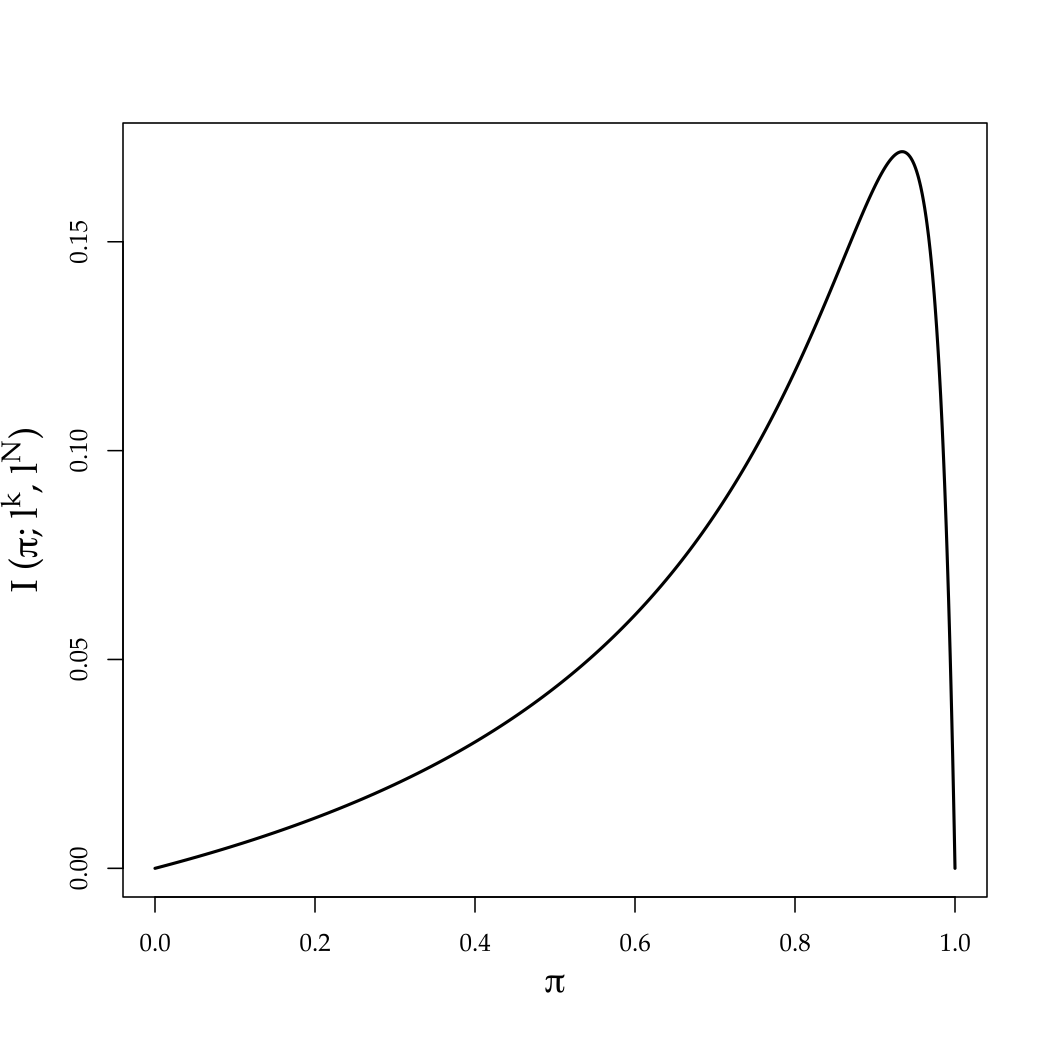
When a sender can only receive two pieces of evidence (so $K=3$), then as Sender 1 would never disclose the “low” signal $s^1$ ($b$ earlier), the only signal that would be disclosed is $s^K$ ($g$ earlier), which necessarily has $l^K>1$. In this case, the right-hand side of Equation 8 is negative, so that ${𝔼}_{\tilde{\pi }}[I(\tilde{\pi };l^K,l^N)]$ is concave over the entire domain $\tilde{\pi }\in (0,1)$. More generally, however, one is only assured that Sender 1 will disclose the highest signal $s^K$ and conceal the lowest signal $s^1$; some intermediate evidence $s^k$ with could be disclosed. The key point is that Lemma 2 does not depend on the number of signals, as Proposition 3 shows that Lemma 2 holds beyond binary signal structures. From the point of view of expected impact, one can view Lemma 2 as showing that, in general, whereas the expected impact of disclosing any particular evidence can be larger in a multi-sender environment (compared to a single-sender environment), the “average” expected impact—averaging over the signals that a sender would disclose—is indeed lower in the multi-sender environment.

A different perspective on why a sender’s influence should be less with two senders is that the DM simply values each sender’s signal less in the presence of another sender. This is also not generally true. In fact, even setting aside any strategic issues, one can construct examples (with binary signals) in which the DM’s expected utility gain (under a quadratic loss function) from obtaining a second signal over the first is larger than the gain from obtaining the first over no signal. An intuition is that the DM’s gain from obtaining a signal can be locally convex in the prior.

5 Conclusion

This article has studied the incentive of biased agents to acquire costly evidence in a persuasion game in which unfavorable information can be strategically concealed. Skeptical, but rational, inference by the decision maker (DM) creates a credible threat that punishes a sender’s non-disclosure with an unfavorable belief, which creates an incentive for the sender to collect evidence even when his preferences are linear over the DM’s belief. There is an equilibrium discrepancy between the sender’s and DM’s beliefs when the sender does not furnish evidence. In particular, when the sender has truly failed to turn up evidence or if he does not disclose favorable evidence, the DM’s belief is overly unfavorable from the sender’s perspective. The sender expects other senders’ disclosure to, on average, “correct” this belief of the DM, no matter the other senders’ biases. Consequently, additional senders reduce an existing sender’s incentive to acquire information: senders’ information acquisition decisions are strategic substitutes.

By implication, the conventional wisdom that competition forces each sender to reveal more information does not hold when endogenous information acquisition is taken into account. The DM may be harmed by the presence of more senders. In a similar vein, a DM’s own investigation may discourage a sender from acquiring information and, as a result, a DM may want to delegate information acquisition to a biased expert or advisor even if it is costless for a DM to acquire a limited amount of information. We refer to the Introduction for applications in which these cautionary results may be relevant.

We conclude by reiterating that our assumption of senders’ preferences being linear in the DM’s belief plays a central role in our analysis. Linearity may be appropriate for some applications (e.g., whenever senders are risk neutral over the DM’s decision, which equals her expectation of the state) or may be justified as a first-order approximation. When senders’ preferences are not linear, they will care about not only how other senders’ messages affect the DM’s expectation—which is what our insights turn on—but also higher-order moments. We are aware that there are specifications under which senders’ information acquisition decisions are not strategic substitutes. Consider an example (with binary conditionally independent signals) in which Sender 1’s preferences over the DM’s belief $\beta$ are represented by the log likelihood ratio $V(\beta )\equiv \log \frac{\beta }{1-\beta }$. The marginal benefit of effort is a generalization of Equation 2:

$$M{B}_1({\widehat{e}}_1,{\widehat{e}}_2)={\mathrm{Pr}}_1[g]{𝔼}_{m_2|g}\left[V({\beta }_{G{m}_2}({\widehat{e}}_2))-V({\beta }_{N{m}_2}({\widehat{e}}_1,{\widehat{e}}_2))\right],$$

where the expectation is taken over $m_2$ given $s_1=g$. Exploiting the form of Bayesian updating of log likelihood ratios, it can readily be checked that the marginal benefit of effort is now independent of ${\widehat{e}}_2$. Thus, for this particular specification, each sender would exert the same amount of effort independent of other senders, and the DM would be strictly better off with every additional sender. Further analysis awaits future research.