Single-Crossing Differences in Convex Environments111Previous versions of this paper were circulated under the title “Single-Crossing Differences on Distributions”. We thank Nageeb Ali, John Duggan, Federico Echenique, Mira Frick, Ben Golub, Ryota Iijima, Ian Jewitt, Alexey Kushnir, Shuo Liu, Daniele Pennesi, Jacopo Perego, Lones Smith, Bruno Strulovici, and various audiences for helpful comments.
Abstract
An agent’s preferences depend on an ordered parameter or type. We characterize the set of utility functions with single-crossing differences (SCD) in convex environments. These include preferences over lotteries, both in expected utility and rank-dependent utility frameworks, and preferences over bundles of goods and over consumption streams. Our notion of SCD does not presume an order on the choice space. This unordered SCD is necessary and sufficient for “interval choice” comparative statics. We present applications to cheap talk, observational learning, and collective choice, showing how convex environments arise in these problems and how SCD/interval choice are useful. Methodologically, our main characterization stems from a result on linear aggregations of single-crossing functions.
Keywords: monotone comparative statics, choice among lotteries, interval equilibria, aggregating single crossing
1 Introduction
1.1 Overview
Single-crossing properties and their implications for choices are at the heart of many economic models, as highlighted by Milgrom and Shannon (1994). Consider a utility function , where is the choice object and a preference parameter. In this paper, we completely characterize the structure of when it has single-crossing differences in a rich—specifically, convex—environment. Before defining this property more precisely and explaining our results, we begin with some background and motivation for our work in a leading context: choice among lotteries.
Motivation.
In various applications of single crossing, choices have been restricted to deterministic outcomes when it would be desirable to accommodate lotteries. Consider Crawford and Sobel’s (1982) canonical cheap-talk model: a sender with private type chooses a costless message to send a receiver, who then takes a decision . A single-crossing property on the sender’s utility ensures that any equilibrium is an “interval equilibrium”, i.e., is partitioned into intervals that induce the same decision. This result is predicated on assumptions ensuring that in equilibrium, the sender can fully anticipate the decision induced by each message. However, in assorted contexts, one would like to model a sender who is uncertain about the receiver’s preferences; but then, from the sender’s perspective, each message would induce a lottery over decisions.
A challenge with extending single-crossing properties to choice among lotteries is that there is no natural order on the set of all lotteries. Moreover, it is not always apparent a priori what restrictions are reasonable on the set of feasible lotteries, in particular whether some form of stochastic dominance can order every choice set an agent may face. In the cheap-talk problem, the nature of the receiver’s preferences may well imply that a higher message (in equilibrium) induces lotteries that have both higher mean and higher variance. In other applications, the lotteries may be the result of still further interactions—e.g., they may represent continuations in dynamic strategic problems—that are intractable to structure ex ante.
An alternative to restricting the set of lotteries is to require that an agent’s utility difference between any pair of lotteries—or, more abstractly, any pair of choice objects—is single crossing in the agent’s preference parameter or type. (For any ordered set , a function is single crossing if its sign is monotonic.) It is this single-crossing property that we study, which we refer to as single-crossing differences (SCD). Our notion is closely related to that of Milgrom and Shannon (1994) for comparative statics, and the “order restriction” property Rothstein (1990) introduced for collective choice. As we explain in Section 2, SCD characterizes interval choice (Theorem 1), a fundamental property for applications. Loosely, interval choice says that given any choice set and any alternative in that set, if a low and a high type both find that alternative optimal, then so do all intermediate types. In the cheap-talk application, the sender’s alternatives are messages, and interval choice yields the aforementioned interval equilibrium desideratum.
A key question, then, is: for an expected-utility agent, which (von Neumann Morgenstern) utility functions assure SCD over lotteries? It is not enough that SCD holds over pure outcomes:
Example.
Let , , and for while . For any , is single-crossing in as its sign does not depend on . But for the uniform lottery over outcomes and , the expected utility difference is not single crossing in . Hence, has SCD over pure outcomes but does not have SCD over lotteries.
SCD in Convex Environments.
In the foregoing example, SCD holds for “extreme” alternatives (i.e., pure outcomes) but fails over “in-between” alternatives (i.e., lotteries). We find this broader viewpoint valuable, as various economic settings have such richness in the alternatives. Accordingly, consider a utility function , where is an action (i.e., a choice alternative) and the ordered type. Say that the choice environment is convex if the set of functions is convex.222That is, for all and , there is such that for all , .
Convex choice environments abound. The function can be expected utility and the set of lotteries over arbitrary outcomes. But, as explained by Example 2 in Section 3, can also be rank-dependent utility (Quiggin, 1982). Or, as detailed in Example 3, can be a product set representing different dimensions of the choice object, and can be a multidimensional utility function with convex range. This class captures examples of deterministic settings in mechanism design, dynamic consumption streams, and choices over bundles of goods or products with multiple characteristics.
Our paper’s main result, Theorem 2, is a characterization of SCD in any convex environment. Theorem 2 establishes that in a convex environment, has SCD if and only if
| (1) |
where and are single-crossing functions that satisfy a ratio-ordering property we define in Section 3. Roughly speaking, ratio ordering requires that the relative importance placed on versus changes monotonically with type.333In particular, if either or is strictly positive, then ratio ordering reduces to saying that the ratio of the two functions is monotonic. More generally, Lemma 1 establishes that ratio ordering is necessary and sufficient for all linear combinations of two single-crossing functions to be single crossing. The idea is transparent when has a minimum and a maximum . Then, having SCD is equivalent to the existence of a (type-dependent) representation that satisfies
where is increasing (Proposition 1). In other words, in such a convex environment, SCD is equivalent to being able to represent each type’s preferences by a utility function that is a convex combination of those of the extreme types, with higher types putting more weight on the highest type’s utility.
In the context of expected utility, there are canonical (von Neumann Morgenstern) functional forms that induce SCD over lotteries: in mechanism design and screening, , where is the quantity, is the transfer, and is the agent’s marginal rate of substitution; in optimal delegation without transfers, , where is the allocation, is money burning, and is the agent’s type (cf. Amador and Bagwell, 2013); in communication/delegation and voting, , where is an outcome and is the agent’s bliss point. On the other hand, our characterization also makes clear that SCD is quite stringent. For example, within the class of power loss functions, only the quadratic loss function generates SCD over lotteries (Corollary 2). Outside of expected utility, we explain in Subsection 3.2 when discounted utility and Cobb-Douglas utility satisfy SCD in a convex environment; in particular, it holds for the simple two-good case of , where are the quantities and parameterizes the marginal rate of substitution.
Applications.
Section 4 applies SCD in convex environments to three economic problems, highlighting the implications of interval choice. Among other things, the cheap-talk application with uncertain receiver preferences in Subsection 4.1 demonstrates concretely how choices from all lotteries emerge naturally. In Subsection 4.2’s observational-learning application, a convex environment stems from multidimensional utility. Subsection 4.3 considers collective choice over lotteries, showing how our results contribute to a long-standing question of whether equilibrium exists when political candidates can offer lottery platforms (Zeckhauser, 1969; Shepsle, 1972).
1.2 An Intuition
A key step towards Theorem 2’s characterization of SCD in convex environments is establishing that every type’s utility is an affine combination of two (type-independent) functions: Equation 1. We can provide a succinct intuition when has a minimum and a maximum . It suffices to show that there are three actions, , , and , such that any type ’s utility from any action satisfies
| (2) |
for some with . (Equation 1 follows by setting, for , , , and .) The desired is the solution to
which exists at least when there are three actions for which the matrix on the right-hand side is invertible. To interpret this matrix equation, note that in a convex environment, any convex combination of utilities from is the utility from some action. Hence, the equation says that one can find two distinct actions with utilities equal to convex utility combinations of such that the lowest and highest types are both indifferent between those two actions.444Take one utility combination to be that corresponding to the uniform distribution on and the other corresponding to for any sufficiently small . By SCD, all types must be indifferent between these two actions, which amounts to Equation 2.
A second key step towards Theorem 2 is showing that the two type-independent utilities in Equation 1 must be ratio ordered. The intuition for this step is provided in Subsection 3.3.
1.3 Related Literature
We now offer a summary of related work, supplying additional details later.
Quah and Strulovici (2012) consider an expected-utility agent choosing under uncertainty about her preferences, which depend on some unknown “state”. They ask when single-crossing differences in the Milgrom and Shannon (1994) sense is preserved regardless of the state distribution. In our expected-utility application, we consider an agent who knows her preferences but chooses among lotteries. Although these are conceptually different questions, there is a mathematical connection in portions of our analysis. Quah and Strulovici’s (2012) question concerns when single crossing is preserved by positive linear combinations. On the other hand, our problem turns on arbitrary linear combinations preserving single crossing. As elaborated after Lemma 1, this explains the difference between Quah and Strulovici’s signed-ratio-monotonicity condition and our ratio-ordering condition. Moreover, there is no analog in their analysis to the linear dependence we deduce in Proposition 2, which is crucial to our main characterization’s functional form (5).
When , the utility specification induces expected utility with SCD over lotteries; indeed, the expected-utility difference between any two lotteries is monotonic in . The usefulness of this utility specification (or slight variants) to structure choices among arbitrary lotteries has been highlighted by Duggan (2014), Celik (2015), and Kushnir and Liu (2018). In Subsection 5.1, we show how SCD preferences always have such a “monotonic differences” representation in convex environments that satisfy a reasonable additional condition. This is a striking consequence of convex environments, as we are not aware of any such result more generally.
In the operations research literature, there has been interest in functional forms for “multi-attribute utility functions” (e.g., Fishburn, 1974). When there are two attributes and the agent has expected-utility preferences, Abbas and Bell (2011) study a “one-switch condition” that is akin to SCD over lotteries on one attribute. In that setting, they offer a result related to our Proposition 1. However, they do not identify ratio ordering as the property that characterizes when single crossing is preserved under aggregation, which is a key contribution of our analysis (Lemma 1 and Proposition 2). Also novel to our paper are the comparative statics characterizations of SCD (Theorem 1 and Theorem 4) and our economic applications.
For choice among restricted sets of lotteries (which we wish to largely avoid, for reasons mentioned earlier), there are various prior results on the conditions for monotone comparative statics under expected-utility preferences. Standard restricted classes of lotteries include those ordered by first-order stochastic dominance (Topkis, 1978) and likelihood-ratio dominance (Karlin, 1968; Athey, 2002).555For first-order stochastic dominance, the requirement is that the utility function is supermodular; for likelihood-ratio dominance, it is log-supermodularity. Smith (2011) considers choice among arbitrary lotteries and their certainty equivalents.
Outside of expected utility on lottery spaces, we are not aware of any work highlighting SCD in convex environments. In our view, the lens of convex environments is a contribution of our paper.
2 Single-Crossing Differences and Interval Choice
Our analysis begins by formalizing comparative statics results that justify a notion of single-crossing differences without reference to an order over the choice space.
Let be a (partially) ordered set containing upper and lower bounds for all pairs.666A partial order—hereafter, also referred to as just an order—is a binary relation that is reflexive, anti-symmetric, and transitive (but not necessarily complete). An upper (resp., lower) bound of is (resp., ) such that (resp., ) for all . While none of our results require any assumptions on the cardinality of , the results in Section 3 are trivial when . See an earlier version of this paper, Kartik et al. (2019, Appendix I), for how our results extend when is only a pre-ordered set, i.e., when does not satisfy anti-symmetry. We often refer to elements of as types.
Definition 1.
A function is:
-
1.
single crossing (resp., from below or from above) if is monotonic (resp., increasing or decreasing);777For , if , if , and if . A function is increasing (resp., decreasing) if (resp., ); it is monotonic if it is either increasing or decreasing. An equivalent, and perhaps more familiar, definition of being single crossing from below is .
-
2.
strictly single crossing if it is single crossing and there are no such that .
Definition 2.
Given any set , a function has:
-
1.
single-crossing differences (SCD) if , the difference is single crossing in ;
-
2.
strict single-crossing differences (SSCD) if such that , is strictly single crossing in .
Our definition of (S)SCD is related to but different from Milgrom and Shannon (1994), who stipulate that has (strict) single-crossing differences given an order on if for all , is (strictly) single crossing from below. (Here, is the strict component of . Note that the (S)SCD terminology is due to Milgrom (2004).) We do not presume that is ordered, but we consider differences for all pairs of elements of . For an arbitrary complete order on , our definition is weaker than Milgrom and Shannon’s (1994) because ours does not constrain the direction of single crossing; on the other hand, it can be checked that our definition implies theirs for a suitably chosen order on that is largely complete.888The order, and the sense in which it is largely complete, is elaborated around Theorem 4 in Subsection 5.2. As established below, our notion characterizes related but distinct comparative statics from Milgrom and Shannon’s.
Our notion of SCD is also closely related to Rothstein’s (1990) notion of order restriction, which he introduced in the context of collective choice. Like SCD, order restriction does not presume an order on the choice space. Order restriction is more permissive insofar as the order on the type space can be chosen to generate SCD; it is more restrictive in requiring that order to be complete.
Interval Choice.
We say that is an interval if and imply . Let with for each and . We say that has interval choice if is an interval for each and . That is, interpreting as a choice correspondence, the set of types choosing any alternative given any choice set is an interval. We say that strictly violates SCD if there are and such that .
Theorem 1.
Let and for any and .
-
1.
If has SCD, then the choice correspondence has interval choice. If strictly violates SCD, then does not have interval choice.
-
2.
If , then has SSCD if and only if every selection from has interval choice.
The intuition for the sufficiency of (S)SCD in Theorem 1 is straightforward. Regarding necessity, we note that a violation of SCD—as opposed to a strict violation—is compatible with the choice correspondence having interval choice: e.g., , with , and .999On the other hand, a strict violation of SCD is slightly stronger than needed: one could weaken its requirement to . Our formulation with both inequalities being strict amounts to putting aside indifferences, which proves convenient for the applications in Section 4. In Part 2 of the theorem, if then any selection from any choice correspondence trivially has interval choice, yet does not have SSCD when for some and all .
Monotone Comparative Statics.
Our choice space is unordered. Intuitively, interval choice is intimately related to there being monotone comparative statics (MCS)—i.e., in some sense, higher types make higher choices—with respect to some complete order on the choice space. We formalize this connection in Subsection 5.2 by tying (S)SCD to MCS. In brief, given any order on , we order subsets of by the corresponding strong set order, and say that the function has MCS if, for every choice set and all types , the higher type chooses a higher set: . Roughly speaking, Theorem 4 in Subsection 5.2 shows that an order on induces MCS if and only if has SCD and the order is a refinement of a natural “SCD-order” generated by .
3 Single-Crossing Differences in Convex Environments
This section characterizes single-crossing differences in “rich” environments. We now assume the existence of a strictly increasing real-valued function on .101010That is, we assume such that . This requirement is related to utility representations for possibly incomplete preferences (Ok, 2007, Chapter B.4.3). A sufficient condition is that has a countable order dense subset, i.e., there is a countable set such that (Jaffray, 1975, Corollary 1). The assumption only plays a technical role in establishing our characterization of strict SCD, i.e., in the second statement of Theorem 2. This requirement is satisfied, for example, when is finite, or is endowed with the usual order. We assume the environment is convex in the following sense:
| () |
That is, a convex environment is rich enough insofar as for any pair of actions and any weighting, there is a third action that replicates the weighted sum of utilities of the original actions. We stress that convexity is in terms of utilities: we have not assumed any structure on . However, if is convex, then it is straightforward that () is assured by linearity of in its first argument.
Example 1 (Expected Utility).
Consider an expected-utility agent who chooses among lotteries. There is a set of consequences and the agent has utility . Letting be the set of all finite-support lotteries over , the agent’s utility from lottery is given by .111111We restrict attention to finite-support distributions throughout the paper for ease of exposition, as it guarantees that expected utility is well defined no matter the distribution and utility function. Nevertheless, we write integrals rather than summations when it simplifies notation regarding the domain of integration/summation. This is a case in which Condition () holds because is linear in its first argument and is convex.
Example 2 (Rank-Dependent Expected Utility).
Continuing with lotteries, non-expected utility environments can also be convex. By virtually the same logic as above for expected utility, it is sufficient for () that the utility from lottery be given by , with an arbitrary reweighting function whose image is convex. For example, a standard formulation of rank-dependent utility (Quiggin, 1982; Diecidue and Wakker, 2001) corresponds to with , and a strictly increasing function satisfying and such that for any lottery and consequence , the reweighting is given by , where is the probability mass function of the lottery . So long as is continuous, has a convex image as required; the image is simply .
Example 3 (Multidimensional Utility).
While lotteries naturally induce a convex environment, they are not necessary. Another example is choice among multidimensional actions. Specifically, and for any , utility is given by for some pairs of functions , with each having a convex image. That is a product set and each has a convex image ensures (). We refer to this specification as multidimensional utility.
Here are some economic contexts in which there is multidimensional utility. First, a consumer chooses among products with multiple characteristics or a bundle of multiple goods, denoted . Each characteristic or good with quality or quantity has a common value , but the tradeoff across characteristics/goods varies with the consumer’s preference parameter , as given by . Second, a designer uses an incentive-compatible direct mechanism that maps an agent’s private type to an action . The designer’s payoff is , where is the designer’s utility from allocating to , and is a type distribution that depends on some parameter . Third, an agent chooses consumption in each period . The agent’s present discounted value is , where is discount function parameterized by .
Example 4 (Experiments).
Our final example is one in which an expected-utility agent can only choose from a proper subset of lotteries. Let be a finite set of “states”. We refer to as the set of beliefs or posteriors and as the set of experiments (with finite support). In Bayesian persuasion (Kamenica and Gentzkow, 2011) or, more broadly, information design (Bergemann and Morris, 2019), an expected-utility agent has preferences represented by , where and is a preference parameter. The expected utility from experiment is given by . If we consider all experiments, then this setting is a special case of Example 1. But given a prior , any experiment must in fact be Bayes-plausible, i.e., its distribution of posteriors must average to the prior . So, given , the agent can only choose an experiment in . Nevertheless, the linearity of in its first argument and the convexity of again imply (). Indeed, based on Example 2, Condition () will hold even for rank-dependent expected-utility agents choosing among Bayes-plausible experiments.
3.1 The Characterization
Our characterization of SCD in convex environments (Theorem 2 below) requires the following definition.
Definition 3.
Let each be single crossing.
-
1.
ratio dominates if
(3) (4) -
2.
strictly ratio dominates if Condition (3) holds with strict inequality.
-
3.
and are (strictly) ratio ordered if either (strictly) ratio dominates or vice-versa.
Condition (3) contains the essential idea of ratio dominance and is what we focus on in the main text; Condition (4) only deals with some knife-edged cases that are discussed in Appendix B.1. The definition of strict ratio dominance does not make reference to Condition (4) because that condition is vacuous when Condition (3) holds with strict inequality.
We use the terminology “ratio dominance” because when is a strictly positive function, Condition (3) is the requirement that the ratio must be increasing in . Indeed, if both and are probability densities of random variables and , then (3) says that stochastically dominates in the sense of likelihood ratios.121212From the viewpoint of information economics, think of as a signal of a state , drawn from the density . Condition (3) is Milgrom’s (1981) monotone likelihood-ratio property for .
Condition (3) is a natural generalization of the increasing ratio property to functions that may change sign. To get a geometric intuition, suppose strictly ratio dominates . Let . For every , implies that the vector moves to through a rescaling of magnitude and a clockwise—rather than counterclockwise—rotation (throughout our paper, a “rotation” must be no more than degrees).131313To elaborate on the direction of rotation, recall that from the definition of cross product, where is the counterclockwise angle from to , , is the cross product, and is the Euclidean norm. If (resp., ), then moves to through a clockwise (resp., counterclockwise) rotation.
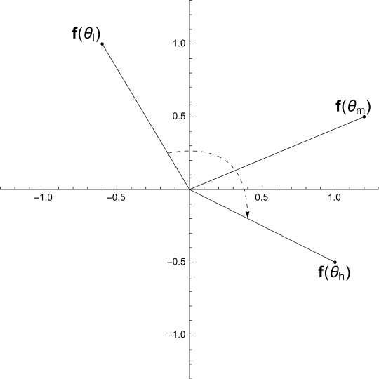
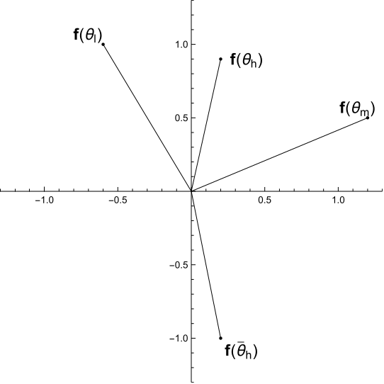
Hence, and are ratio ordered only if rotates monotonically as increases, either always clockwise or always counterclockwise.141414The preceding discussion establishes this point under the presumption of strict ratio ordering; however, because of the hypothesis in Definition 3 that and are single crossing and because of Condition (4), the conclusion holds for ratio ordering too. Furthermore, it can be confirmed that a monotonic rotation of implies ratio ordering if there are no and such that and are collinear. It follows that the set must be contained in a closed half-space of defined by a hyperplane that passes through the origin: otherwise, there will be two pairs of vectors such that an increase in corresponds to a clockwise rotation in one pair and a counterclockwise rotation in the other. See Figure 1. In its panel 1(b), the non-monotonic rotation of is clear when with , but it is also present when with ; in the latter case, the aforementioned half-space requirement is violated.
We can now state our main characterization. For brevity, we say that has (S)SCD⋆ as shorthand for “In a convex environment, has (S)SCD.” Furthermore, we say that is minimal if there is no pair of utility-indistinguishable actions: , such that .
Theorem 2.
The function has SCD⋆ if and only if it takes the form
| (5) |
with and each single crossing and ratio ordered. In addition, if is minimal, then has SSCD⋆ if and only if and are strictly ratio ordered.151515If is not minimal, then so long as , violates SSCD⋆ because for some and ’, is a zero function and hence not strictly single crossing. Nonetheless, the characterization applies when we consider utility-indistinguishable actions as equivalence classes and the corresponding utility function on those equivalence classes.
We make a number of observations to help interpret Theorem 2.
The theorem says that for to have SCD⋆, it must be possible to write it in the form (5). Notice that given (5), for any , the function is a linear combination of and . Therefore, to rule out the possibility of the form (5), it is sufficient to find and such that the matrix is invertible. This procedure is often useful to reject SCD⋆, as we illustrate subsequently in Corollary 2.
Given the functional form (5), not only is SCD⋆ assured by and each being single crossing and ratio ordered, but these properties are almost necessary.161616“Almost” excludes the case in which and are affinely dependent, i.e., for some . Intuitively, affine independence ensures that neither nor is dispensable in (5).
An asymmetry between and in Equation 5 bears noting: the function does not have a counterpart function . The reason is that whether the utility difference between two actions is single crossing could be altered by adding a function of alone to . On the other hand, adding a function of alone has no such effect because SCD is an ordinal property that is invariant to any (type-dependent) increasing transformation, or representation, of , i.e., , where each is strictly increasing.
In general, whether the convexity condition () holds can depend on which representation one chooses. But since SCD is ordinal, the scope of our analysis is in fact broader than it may seem: if a utility function satisfies SCD and some representation satisfies (), then Theorem 2 applies to that representation.171717For example, given a product set and , the Cobb-Douglas utility does not satisfy (), but the representation is a multidimensional utility (Example 3) and therefore satisfies (), indeed SCD⋆. We illustrate how this is useful in Subsection 3.2.3.
If has the form (5) with strictly positive functions and , then up to a positive affine transformation (viz., subtracting and dividing by ),181818In general, a positive affine transformation of is any where . Unlike arbitrary representations, positive affine transformations preserve condition (). any type’s utility becomes a convex combination of two type-independent utility functions over actions, and . Theorem 2’s ratio ordering requirement then simply says that the relative weight on and changes monotonically with the agent’s type. This idea underlies the following proposition.
Proposition 1.
Let have both a minimum and a maximum (i.e., such that ), and the environment be convex. Then, has SCD⋆ if and only if has a positive affine transformation satisfying
| (6) |
with increasing. In addition, if is minimal, then has SSCD⋆ if and only if is strictly increasing.
Proposition 1 provides an economic interpretation of SCD⋆ as capturing preferences that monotonically shift weight from one extreme type’s to the other’s. We note, though, that even when has extreme types, it could be easier to verify whether a given function has SCD⋆ using Theorem 2 because one does not have to search among the affine transformations allowed by Proposition 1.
We offer one additional interpretational comment. On the one hand, Theorem 2 and Proposition 1 indicate that SCD—while desirable for tractability (including interval choice), economic intuition, etc.—is a demanding property in a convex environment. On the other hand, because the functions and in Theorem 2 are arbitrary, SCD⋆ nevertheless allows for a broad economic landscape. Specifically, when one assumes SCD in any environment (convex or not), one generally has in mind that there is an underlying tradeoff—e.g., risk vs. expected return among lotteries, delay vs. total amount in payment streams, or price vs. product quality in markets—whose balance shifts monotonically with type. Our characterizations show that SCD⋆ is broad enough to capture such desiderata because the and functions in Theorem 2 can evaluate the tradeoff differently: e.g., compared to , the function can be more risk averse, discount the future more, or be more price sensitive; furthermore, as highlighted by Proposition 1, higher types put more weight on one criterion.
3.2 Implications for Leading Examples
This subsection develops the implications of Theorem 2 for our leading examples. For brevity, we focus on the implications of SCD⋆, stating the SSCD⋆ counterpart only in Corollary 1.
3.2.1 Single-Crossing Expectational Differences
Suppose, following Example 1, that is a set of lotteries and is the expected utility induced by . We say that has (strict) single-crossing expectational differences, or (S)SCED, if the expected utility function has (S)SCD⋆.191919In general, an expected utility function may not have SSCD⋆ simply because is not minimal. This arises, for example, when is a mean-variance utility function and multiple lotteries have the same mean and variance. In such cases we consider utility-indistinguishable lotteries as equivalence classes and the corresponding utility function defined on these equivalence classes of lotteries. We say has SSCED if has SSCD⋆. SCED is not implied by SCD or even supermodularity of .202020For instance, given , any power loss function is supermodular when , but Corollary 2 below establishes that SCED fails for . Rather:
Corollary 1.
The von Neumann Morgenstern utility function has (S)SCED if and only if it has the same form as in Theorem 2.
The corollary’s proof is straightforward: if satisfies the characterization, then with and satisfying the conditions given in Theorem 2, so has SCD⋆. Conversely, if has SCD⋆, and hence has the form in Theorem 2, then so does because , where denotes the degenerate lottery on .
Corollary 1 is related to Abbas and Bell (2011, Theorem 1). They study expected utility over lotteries with some additional restrictions on the environment (e.g., is finite and completely ordered, and preferences satisfy some substantive economic conditions). For that setting, their Theorem 1 states a similar result to the version of Corollary 1 that would obtain using Proposition 1 instead of Theorem 2.212121Abbas and Bell (2011) use the terminology of “one-switch independence”, which appears equivalent to SSCED up to one minor detail that can be set aside here (concerning the treatment of distinct lotteries that all types are indifferent over). Translated into our notation, they assert that a utility function has SSCED if and only if , with strictly positive and strictly increasing. This can be seen from our Proposition 1 because, given its hypothesis of extreme types, it implies that has SSCED if and only if , where is strictly positive, is strictly increasing, and and are, respectively, monotonic transformations of and .
Even aside from the ratio-ordering and single-crossing requirements in Theorem 2, the functional form (5) deserves emphasis: there are only two “interaction terms”, each of which is multiplicatively separable in and . This means that preferences over lotteries must be summarized by two linear statistics: for any lottery , the statistics are and .222222The utility function cannot be written in the form of Equation 5 and hence does not have SCED. Indeed, its expected utility from an arbitrary lottery cannot be summarized by any finite number of linear statistics, let alone two. This point underlies the following corollary, which identifies quadratic loss as the unique power loss function that has SCED.
Corollary 2.
Let and with . A loss function with has SCED if and only if .
Under quadratic loss, preferences over lotteries are summarized by the lotteries’ first and second moments. We note that some non-power-loss generalizations of quadratic loss, such as with , also satisfy SCED; these functional forms—or variants that also augment a quasilinear money burning component, which continues to preserve SCED—are used in the study of delegation with stochastic mechanisms or money burning (Amador and Bagwell, 2013; Kleiner, 2022).
SCED is useful in dynamic problems, as seen in Banks and Duggan (2006), Duggan (2014), Celik (2015), and Ali et al. (2022). It is thus noteworthy that:
Corollary 3.
Suppose has SCED. Then, denoting , so does the discounted utility function for any .
We omit a proof as the result follows straightforwardly from Corollary 1. Note that Corollary 3 does not require exponential discounting. (Of course, implicitly must ensure that is finite.)
3.2.2 Single-Crossing Rank-Dependent Expected Utility
Suppose an agent’s preferences over lotteries have a rank-dependent expected utility (RDEU) representation as described in Example 2, with underlying utility .
Corollary 4.
An RDEU function has SCD⋆ if and only if the underlying utility has the same form as in Theorem 2.
We omit a proof because it is analogous to that for Corollary 1. An RDEU agent thus evaluates a lottery according to two summary statistics: and . The difference with expected utility is that these summary statistics are no longer linear in . Instead the statistics reweight probabilities according to the original reweighting function.
3.2.3 Multidimensional Utility
Suppose, following Example 3, that an agent has a multidimensional utility function .
Corollary 5.
A multidimensional utility function has SCD⋆ if and only if
| (7) |
with and each single crossing and ratio ordered, and .
The interpretation is that a multidimensional utility has SCD⋆ when at most two “summary” dimensions matter. The values on these summary dimensions are weighted sums of the original values over the primitive dimensions . Higher types place relatively more weight on products/bundles that are more valuable on one of the two summary dimensions; recall Proposition 1.
As mentioned in Example 3, multidimensional utility can capture a consumer choosing among consumption bundles. A canonical specification is the Cobb-Douglas utility , where is the consumption bundle and the vector of parameterizes the consumer’s marginal rates of substitution (MRS). Note that an alternative representation is , which has the multidimensional form. Corollary 5 implies that for Cobb-Douglas utility to have SCD, it must be representable as
with monotonic and .232323More precisely, Corollary 5 yields the representation , where and are each single crossing and ratio ordered, and Proposition 1 yields the further simplification. The interpretation is that to satisfy SCD, the Cobb-Douglas utility must have “two layers”: the consumer first evaluates the -independent Cobb-Douglas value of two composite goods, and then trades off these composite goods according to a Cobb-Douglas utility function with MRS that is monotonic in . SCD guarantees that for any choice set (e.g., a budget set), the value of each composite good in the chosen consumption bundle changes monotonically (necessarily in opposite directions) in . A special case is the textbook example of two goods, say and , and with . In that case, we recover the textbook observation that given any budget set, the consumption of each good is monotonic in the MRS.
As another example, consider discounted utility over consumption streams. For a consumption stream , the discounted utility is of the multidimensional form. Corollary 5 implies that the discounted utility has SCD⋆ only if, for any consumption stream , is linearly generated by two functions of . By considering consumption streams that are positive only in a single period, we see that each must in fact be generated by the same two functions of , i.e., . When , such linear dependency does not hold for exponential discounting, i.e., when each type has a discount factor such that . Consequently, exponential discounting is incompatible with interval choice: given any three discount factors, there are consumption streams and such that an agent with either low or high patience strictly prefers while an agent with intermediate patience strictly prefers .242424For example, let and . The difference is strictly positive if and only if . In fact, our analysis reveals that in general choice between an arbitrary pair of consumption streams will be monotonic in the time preference parameter only if has the aforementioned linear dependence. An example is linear time cost, say and for some .252525The fact that SCD imposes strong restrictions on the nature of discounting can be related to difficulties in aggregating time preferences (Jackson and Yariv, 2015). Specifically, with three types (or agents), , where “” stands for Planner, SCD is very similar to a Pareto principle: whenever types and have the same preference over a pair of consumption streams, so should type . Our discussion indicates that if types and are exponential discounters, then cannot be, as was highlighted by Jackson and Yariv (2015). In fact, our result says that ’s preference must linearly depend on the other two types, echoing Harsanyi (1955).
3.2.4 Single-Crossing Expectational Differences over Experiments
Suppose, following Example 4, that , , and are a set of states, posteriors, and experiments respectively. Given a prior , an agent can only choose a Bayes-plausible experiment: . We say that has single-crossing expectational differences over experiments (SCED-X) if the expected utility function over has SCD⋆. Since , SCED is sufficient for SCED-X but not necessary. SCED-X is, instead, characterized as follows.
Corollary 6.
For any full-support prior , the function has SCED-X if and only if
| (8) |
with and each single crossing and ratio ordered.
As the environment is convex, Theorem 2’s characterization applies to the expected utility function . Similar to the SCED characterization in Corollary 1, the form of the expected utility function passes to the von Neumann Morgenstern utility function .262626This is not as straightforward as in the case SCED, where one can appeal to degenerate lotteries on any posterior. Under SCED-X, the only posterior on which there can be a degenerate lottery is the prior. The difference is that the last term in Equation 8 can depend on the posterior as well as the type , unlike the term in Equation 5. This is because the expected utility having the form in Theorem 2 only imposes, for SCED-X, that the expectation of that term is constant over lotteries that average to the prior, rather than over all lotteries. This means that the term can admit a linear dependence in , as seen in Equation 8.
3.3 Aggregating Single-Crossing Functions
This subsection explains the logic behind Theorem 2; we focus on single crossing here, deferring strict single crossing to Supplementary Appendix SA.2. Owing to the convex environment, the central issue is when linear aggregations of functions are single crossing. Lemma 1 below shows that ratio ordering is the characterizing property when aggregating two functions; Proposition 2 then establishes that when aggregating more than two functions, no more than two can be linearly independent, which leads to Theorem 2.272727Real-valued functions are linearly independent if is not a zero function, i.e., is not everywhere zero.
Lemma 1.
Let . The linear combination is single crossing if and only if and are each single crossing and ratio ordered.
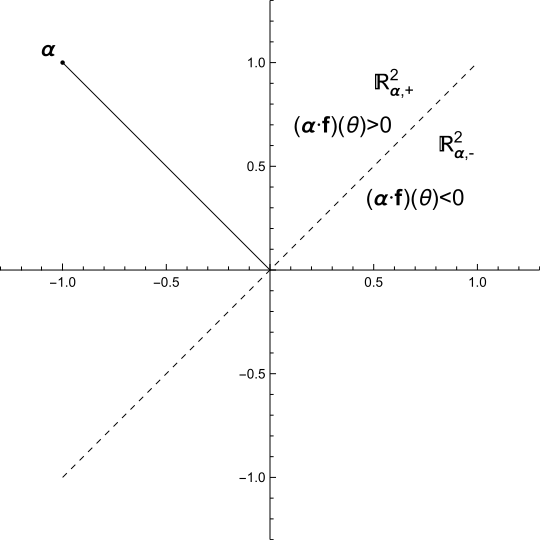
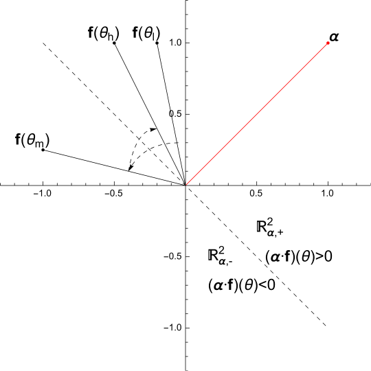
Here is the lemma’s intuition. For sufficiency, consider any linear combination . Assume , to avoid triviality. The vector defines two open half spaces and , where is the dot product; see Figure 22(a). As explained earlier after Definition 3, ratio ordering of and implies that the vector rotates monotonically as increases. If the rotation is from to (resp., from to , then is single crossing only from below (resp., only from above). If or , then is single crossing both from below and above. Other cases are similar.282828Notice that this argument does not require either or to be single signed. By contrast, Abbas and Bell (2011, p. 769, in their last paragraph on “Necessity”) incorrectly claim that all linear combinations of two (strictly) single crossing functions are (strictly) single crossing only if one function is single signed.
To see why Condition (3) of ratio ordering is necessary, suppose the vector does not rotate monotonically. Figure 22(b) illustrates a case in which, for , rotates counterclockwise to , but rotates clockwise to . As shown in the figure, one can find such that while both , which implies that is not single crossing. See Appendix B.1 for why Condition (4) is necessary.
Lemma 1 relates to Quah and Strulovici (2012, Proposition 1). They establish that for any two functions and that are single crossing from below, is single crossing from below for all if and only if and satisfy a condition they call signed-ratio monotonicity (see Supplementary Appendix SA.5 for the definition). In general, ratio ordering is not comparable with signed-ratio monotonicity because we consider a different aggregation problem from Quah and Strulovici: (i) the input functions may be single crossing in either direction; (ii) the linear combinations involve coefficients of arbitrary sign; and (iii) the resulting combination can be single crossing in either direction. The example in the introduction highlights the importance of point (ii). There, and . Both and are positive functions (hence, single crossing from below), and so all positive linear combinations are also positive functions, but is not single crossing because and are not ratio ordered. If the input functions in Lemma 1 are restricted to be single crossing from below, then ratio ordering implies signed-ratio monotonicity.
Lemma 1 implies a characterization of likelihood-ratio ordering for random variables with strictly positive densities. While this likelihood-ratio ordering characterization does not appear to be well-known among economists, it is a special case of Karlin’s (1968) results on the variation diminishing property of totally positive functions. More generally, however, Lemma 1 differs from Karlin (1968) because it considers aggregations of functions that can change sign, whereas he only studies non-negative functions.292929Under some conditions, it is possible to transform the lemma’s aggregation problem into one of aggregating non-negative functions, and then apply Karlin’s (1968) results. However, the precise conditions are opaque (Kartik, Lee, and Rappoport, 2019, Appendix H.2); moreover, the procedure is somewhat involved and, in our view, less instructive than our direct proof of Lemma 1.
Theorem 2 requires an extension of Lemma 1 to more than two functions. Consider any set and . We say that is linear combinations SC-preserving if is single crossing in for every function with finite support.303030The notation should be read as .
Proposition 2.
Let for some set . The function is linear combinations SC-preserving if and only if there exist and such that
-
1.
and are (i) each single crossing and (ii) ratio ordered, and
-
2.
.
Proposition 2 says that a family of single-crossing functions preserves single crossing of all finite linear combinations if and only if the family is “linearly generated” by two single-crossing functions that are ratio ordered. In particular, given any three single-crossing functions, , , and , all their linear combinations will be single crossing if and only if there is a linear dependence in the triple, say for some , and and are ratio ordered.
The sufficiency direction of Proposition 2 follows from Lemma 1, as does necessity of the “generating functions” being ratio ordered. The intuition for the necessity of linear dependence is as follows. Assume is completely ordered. For any , let . If is linearly independent, then there exist such that spans . Take any that is orthogonal to the plane that is spanned by and , as illustrated in Figure 3. The linear combination is not single crossing because while .
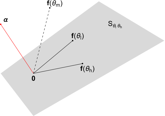
While the necessity portion of Proposition 2 only asserts ratio ordering of the “generating functions”, Lemma 1 implies that if is linear combinations SC-preserving, then for all , the pair and must be ratio ordered.
Proof Sketch of Theorem 2.
We can now sketch the argument for Theorem 2. That its characterization is sufficient for SCD⋆ is straightforward from Lemma 1. For necessity, suppose as a simplification that, for some , .313131This is just a normalization, since has SCD⋆ if and only if has SCD⋆. For any and , we build on the Hahn-Jordan decomposition of to write the linear combination as , where and are probability mass functions on , and is a scalar.323232Let . For , set and . If , set and ; if , set and . Let . Finally, for all , set and . (Unless , we have ; the assumption that permits us to assign all the “excess difference” to , as detailed in fn. 32.) Since the environment is convex there exist such that the linear combination is equal to , which is single crossing because has SCD⋆ . Since every such linear combination is single crossing, Proposition 2 guarantees and such that for all , , with and each single crossing and ratio ordered.
Remark 1.
The proof of Theorem 2 is materially no different from that for an expected-utility environment. Indeed, any convex environment can be transformed into another convex environment where is a convex subset of the vector space of functions , and, under mild conditions, Choquet’s Theorem implies that each is an expected utility function. We develop the lens of convex environments for two reasons: (i) to highlight that our characterization is driven only by Condition (), not other properties of expected utility such as linearity or continuity; and (ii) to cover additional economic settings, as in Examples 2–4.
4 Applications
This section illustrates the usefulness of our results in three applications. Interested readers may consult our earlier working paper, Kartik, Lee, and Rappoport (2019, Section 4.3), for another application to costly signaling.
4.1 Cheap Talk with Uncertain Receiver Preferences
There are two expected-utility players, a sender () and a receiver (). The sender’s type is , where is ordered by . After learning his type, chooses a payoff-irrelevant message , where . After observing but not , takes a decision . The sender’s von Neumann Morgenstern utility function is ; the receiver’s is , where is a preference parameter that is unknown to when choosing , and known to when choosing . Note that does not affect the sender’s preferences. The variables and are independently drawn from commonly-known probability distributions.
An example is , , , and . Here the variable captures the receiver’s “type-independent bias” and captures the relative “sensitivity” to the sender’s type. If were commonly known and uniformly distributed, this would be the model of Melumad and Shibano (1991), which itself generalizes the canonical example from Crawford and Sobel (1982) that obtains when and .
We focus on (weak Perfect Bayesian) equilibria in which uses a pure strategy, , and plays a possibly-mixed strategy, .333333Our notion of equilibrium requires optimal play for every (not just almost every) type of sender. The restriction to pure strategies for the sender is for expositional simplicity. Given any , every message induces some lottery from the sender’s viewpoint. An equilibrium is: (i) an interval equilibrium if every message is used by an interval of sender types, i.e., if is an interval; and (ii) sender minimal if for all on-the-equilibrium-path , there is some such that . In other words, sender minimality rules out all sender types being indifferent between two distinct on-path messages.343434In Crawford and Sobel (1982) and Melumad and Shibano (1991), all equilibria are outcome equivalent to sender-minimal equilibria. More generally, all equilibria are sender minimal when there is a complete order over messages under which higher messages are infinitesimally more costly for all sender types.
Claim 1.
If has SSCED (Corollary 1) then every sender-minimal equilibrium is an interval equilibrium.
-
Proof.
From the sender’s viewpoint, the lottery over the receiver’s decisions that is induced by any message (given any receiver strategy) is independent of because and are independent. The result follows from Theorem 1, as sender-minimality implies that one can restrict attention to the sender choosing among lotteries that are utility-distinguishable (i.e., if and are equilibrium lotteries, then is not a zero function). ∎
Claim 1 relates to Seidmann (1990), who first considered an extension of Crawford and Sobel (1982) to sender uncertainty about the receiver’s preferences. His goal was to illustrate how such uncertainty could facilitate informative communication even when the sender always strictly prefers higher receiver decisions. Example 2 in Seidmann (1990) constructs a non-interval and sender-minimal equilibrium that is informative. Claim 1 clarifies that the key is a failure of SSCED.
The strict single-crossing property in standard cheap-talk models (e.g., Crawford and Sobel (1982) and Melumad and Shibano (1991)) not only yields interval equilibria, but it also implies that local incentive compatibility is sufficient for global incentive compatibility. This additional tractability also holds under SSCED. Let such that for , and be a candidate equilibrium outcome (i.e., the distribution of receiver’s choices that each sender type induces in equilibrium). Under SSCED, it is sufficient for sender incentive compatibility that .
Besides being sufficient, (S)SCED is also necessary to guarantee interval cheap-talk equilibria. Say that strictly violates SCED if the expected utility function strictly violates SCD, i.e., if there are and such that .
Claim 2.
Let , , , and . If strictly violates SCED, then for some pair of distributions of and there is a non-interval equilibrium in which each sender type plays its unique best response.
-
Proof.
Assume strictly violates SCED and let and be the distributions and the types in that definition. In what follows, we can without loss assume . So let and consider the sender’s strategy
Let be any distribution with support and . Then, the unique best response against for a receiver of type is
It can be verified that there is a distribution such that, from the sender’s viewpoint, the message leads to the distribution and the message leads to the distribution , and so is the sender’s unique best response.353535Let and be random variables with distributions and , respectively. Let be the distribution of a random vector defined by As (i.e., has distribution ), is stochastically equivalent to . Thus, and . ∎
The particular specification of in Claim 2 is not critical; what is important is that there be enough flexibility to generate appropriate lotteries from the sender’s viewpoint using best responses for the receiver.363636In particular, the result in Claim 2 holds under the following more general assumptions: , the receiver’s preferences are represented by , and for every and , there exists such that and . The proof is very similar to that of Claim 2. For example, the result would also hold—more straightforwardly, but less interestingly—if the receiver were totally indifferent over all actions for some preference realization. On the other hand, if and , then (S)SCED is not necessary, because any pair of lotteries that the sender may face are ranked by first-order stochastic dominance. Strict supermodularity of then guarantees that all sender-minimal equilibria are interval equilibria; however, strict supermodularity does not imply (S)SCED, as noted in Subsection 3.2.1.
In our cheap-talk application it is uncertainty about the receiver’s preferences that leads to the sender effectively choosing among lotteries over the receiver’s decisions. Similar results could also be obtained when the receiver’s preferences are known but communication is noisy, à la Blume et al. (2007).
4.2 Observational Learning with Multidimensional Utility
The classic sequential observational learning model (Banerjee, 1992; Bikhchandani et al., 1992) considers agents sequentially choosing products with uncertainty about product values but learning from predecessors’ choices.
For concreteness, suppose that students sequentially purchase laptops before entering an engineering school. Each laptop is identified by its attribute vector , which consists of processing power, memory, screen size, price, etc. The students are uncertain about the nature of the work required to complete the degree, which is captured by a state , where is countable. The state affects how students weigh each attribute of a laptop. Specifically, following Example 3, students have a common multidimensional utility function . Each has a convex range, which ensures a convex environment, i.e., Condition (). Students are expected-utility maximizers.
Given a finite set of available laptops and a prior over the state, each student chooses a laptop using two information sources. Conditional on the state, student obtains an independent private signal about (e.g., her own impression from reading syllabi and talking to alumni). A canonical example is normal information: , where is a known constant. Each student also observes all predecessors’ choices.
The question is whether there is adequate learning, as defined by Kartik et al. (2022): no matter the prior and the choice set , do students’ sequential choices eventually settle on the laptop they would choose if the state were known?373737Here is a precise definition. The full-information expected utility given a belief is the expected utility under that belief if the state will be revealed before an action is chosen: Given a prior and a strategy profile , student ’s utility is a random variable. Let be student ’s ex-ante expected utility. There is adequate learning at a choice set if for every prior and every equilibrium strategy profile , as . There is adequate learning if there is adequate learning at all choice sets. Those authors identify SCD as the necessary and sufficient condition on the utility function for learning under normal information, and more generally, for information structures that have “directionally unbounded beliefs”.383838Roughly, an information structure has directionally unbounded beliefs if for every state there exist signals that provide arbitrarily-close-to relative certainty about that state vs. all lower states, and analogously (potentially different) signals for that state vs. all higher states. Under normal information, for any state, arbitrarily high signals deliver the former while arbitrarily low signals deliver the latter. In the current multidimensional utility environment, the following characterization obtains, which we state without proof.
Claim 3.
There is adequate learning under normal information if and only if has SCD⋆, i.e., it has the form stated in Corollary 5.
The claim implies that adequate learning under normal information obtains if only if students’ preferences depend on at most two “summary attributes”, which are each linear combinations over the original value over attributes, i.e., linear combinations of the functions . For example, students may trade off “convenience”, which is an aggregate of price, weight, and size, with “performance”, which aggregates processing speed, memory, and storage. Learning requires that the convenience and performance aggregators do not vary with the state. A second implication derives from and in Equation 7 being ratio ordered. The interpretation is that for learning, students must value one summary attribute more as the state increases, e.g., a higher state indicates more computationally intensive work and hence a higher value of performance relative to convenience.
4.3 Collective Choice over Lotteries
Collective choice over lotteries manifests in many contexts: elections entail uncertainty about what policies elected politicians will implement; and a board of directors may view each candidate for CEO as a probability distribution over firm earnings. Zeckhauser (1969) first pointed out that pairwise-majority comparisons in these settings can be cyclical, even when comparisons over deterministic outcomes are not. Our results shed light on when such difficulties do not arise.
Consider a finite group of individuals indexed by , where for simplicity is odd. The group must choose from a set of lotteries over where is the space of outcomes (political policies, earnings, etc.) with generic element . Each individual has von Neumann Morgenstern utility function , where is a preference parameter or ’s type. We assume is completely ordered; without further loss of generality, let and . The expected utility for an individual of type from lottery is . We denote individual ’s preference relation over lotteries by , with strict component .
Define the group’s preference relation, , over lotteries and by majority rule:
Claim 4.
If has SCED (Corollary 1), then the group’s preference relation is transitive and coincides with that of individual .
The claim follows from the arguments of Rothstein (1990) and Gans and Smart (1996), but we include a direct proof given how short it is.
-
Proof.
Let . By SCD, (i) if , then because there cannot exist such that and ; analogously, (ii) if , then . Hence, coincides with . ∎
Claim 4 can be applied to a well-known problem in political economy (Shepsle, 1972). For simplicity, we now further assume the policy space is a finite set and there is a group of voters whose types are their ideal points, i.e., . There are two office-motivated candidates, and ; each can commit to any lottery from some given set . A restricted set may capture various kinds of constraints; for example, Shepsle (1972) assumed the incumbent candidate could only choose degenerate lotteries. In our setting, what ensures the existence of an equilibrium, and which policy lotteries are offered in an equilibrium?393939More precisely: the two candidates simultaneously choose their lotteries, and each voter then votes for his preferred candidate (assuming, for concreteness, that a voter randomizes between the candidates with equal probability if indifferent). A candidate wins if he receives a majority of the votes. Candidates maximize the probability of winning. We seek a Nash equilibrium of the game between the two candidates.
Claim 4 implies that if voters’ utility functions have SCED and if voter is indifferent between her most-preferred lottery in and in , then there is a unique equilibrium: each candidate offers the best lottery for voter ; in particular, both candidates converge to , the degenerate lottery on , if that is feasible for both. It bears emphasis that in this case policy convergence at the median ideal point is not driven by all voters being globally “risk averse” (e.g., ); rather, it is because SCED ensures the existence of a decisive voter whose most-preferred lottery is degenerate.404040An example may be helpful. Let , , and . The corresponding functions and are each strictly single crossing from below and strictly ratio ordered. For all , is maximized at but is convex on some subinterval of .
There is a sense in which SCED is necessary to guarantee that each candidate will offer the median ideal-point voter’s most-preferred lottery from the feasible set . Suppose strictly violates SCED, i.e., there are and such that . Then, if the population of voters is just and , the unique equilibrium is for both candidates to offer lottery , which is voter ’s less-preferred lottery.
5 Discussion
5.1 Single Crossing vs. Monotonicity
We have characterized when has SCD in a convex environment. SCD is an ordinal property. Analogous to the interest in monotonic functions rather than just single-crossing functions, one may also be interested in the following cardinal property, which we term monotonic differences (MD):
In a convex environment, we write MD⋆ analogously to SCD⋆.
Theorem 3.
The function has MD⋆ if and only if it takes the form
| (9) |
where is monotonic.
Suppose that an expected-utility agent with von Neumann Morgenstern utility is choosing among lotteries, so . We say that has monotonic expectational differences (MED) if the expected utility function has MD⋆. Analogous to the SCED characterization in Corollary 1, it is straightforward that the function has MED if and only if it has the same characterization as given for in Theorem 3. This MED characterization has largely been obtained by Kushnir and Liu (2018) in their study of the equivalence between Bayesian and dominant-strategy implementation.
A function with SCD⋆ has MD⋆ when the function in the form (5) is identically equal to one; and being ratio ordered is then equivalent to being monotonic. In general, SCD⋆ functions need not have MD⋆; however, by Proposition 1, SCD⋆ functions have MD⋆ representations if has both a minimum and a maximum.414141Absent this condition, an SCD⋆ function may not even have an MD⋆ representation. In the context of expected utility, an earlier version of our paper characterized precisely when such representations do not exist and provided an example (Kartik, Lee, and Rappoport, 2019, Appendix G). Duggan (2014, Section 4) also discusses the difficulty of finding SCED functions that do not have MED representations. We view this finding as unexpected; outside of convex environments, we are not aware of any general result on when SCD functions have MD representations.
5.2 Interval Choice and Monotone Comparative Statics
In Section 2, we showed that (S)SCD characterizes interval choice. There is a sense in which interval choice is intimately related to monotone comparative statics holding with respect to some order over the choice space. In light of Theorem 1, the connection is elucidated below by tying (S)SCD to monotone comparative statics.
Throughout this subsection, we consider an ordered set of alternatives, . To simplify exposition and avoid dealing with equivalence classes, we will focus on comparative statics for a function such that is minimal (with respect to ), i.e., . For any , let and denote the usual join and meet respectively.424242Alternative is the join (or supremum) of if (i) and , and (ii) if and , then . The meet (or infimum) of is defined analogously. Neither need exist. Given any , we say that dominates in the strong set order, denoted , if for every and , (i) and exist, and (ii) and . It can be verified that is transitive on non-empty subsets of .
Definition 4.
has monotone comparative statics (MCS) on if
Our definition of MCS is closely related to but not the same as Milgrom and Shannon (1994). We take to be any ordered set while they require a lattice. We focus only on monotonicity of choice in but require the monotonicity to hold for every subset ; Milgrom and Shannon require monotonicity of choice jointly in the pair , but this implicitly only requires choice monotonicity in to hold for every sublattice .
Define binary relations and on as follows: if is single crossing only from below; if either or . It is clear that is reflexive and anti-symmetric. If has SCD, then is also transitive. Moreover, given SCD (and minimality), the order is incomplete only over pairs with “dominance”: if and vice-versa, then either , or .
Theorem 4.
has monotone comparative statics on , where is minimal, if and only if has SCD and is a refinement of .
Our definition of SCD does not require an order on the set of alternatives, whereas MCS does. Theorem 4 says that SCD is necessary and sufficient for there to exist an order that yields MCS. Moreover, the theorem justifies viewing as the prominent order for MCS: MCS does not hold with any order that either coarsens or reverses a ranking by . The argument for necessity in Theorem 4 only makes use of binary choice sets. If SCD fails, then there is no order for which there is choice monotonicity for all binary choice sets. If SCD holds, then choice monotonicity on all binary choice sets requires to refine . For sufficiency in Theorem 4, we show that for any choice set, is a complete order among the set of alternatives that are chosen by some type; thereafter, we appeal to Milgrom and Shannon (1994, Theorem 4).
6 Conclusion
This paper has characterized the class of utility functions that have SCD⋆, i.e., single-crossing differences in a convex environment (Theorem 2). Our notion of SCD does not presume an order on the choice space and is the appropriate notion for interval-choice comparative statics (Theorem 1). We have given a number of examples of convex environments, most notably expected utility, rank-dependent expected utility, and multidimensional utility, and discussed the implications of our characterization in these contexts. The applications in Section 4 illustrate how SCD⋆ is useful in economic problems.
While we have emphasized interval choice, it bears noting that there are other familiar implications of single-crossing properties that in fact rely only on our order-independent notion of (S)SCD; for example, SSCD is the key to guaranteeing that local incentive compatibility implies global incentive compatibility.434343We mean in a sense analogous to Carroll (2012, Proposition 4). While Carroll establishes his result by defining a single-crossing property with respect to some given order over alternatives, essentially the same logic applies with our order-independent notion of strict SCD (Definition 2).
We close by mentioning some avenues for future research. First, it may be of interest to characterize exactly when preferences have a utility representation that satisfies our convexity condition (). Second, and relatedly, one may explore characterizations of SCD outside convex environments. In particular, we are intrigued by the question of when SCD preferences do not possess a representation that takes a similar form to that we have characterized.
Third, our results have direct bearing on problems in which all types of an agent face the same choice set. Such situations are natural. But consider a variation of the cheap-talk application (Subsection 4.1) in which the sender’s type is correlated with the receiver’s type. Even though the receiver’s type does not affect the sender’s payoff, different sender types will generally have different beliefs about the distribution of the receiver’s action that any message induces in equilibrium. Effectively, different sender types will be choosing from different choice sets. An approach that synthesizes the current paper’s with that of, for example, Athey’s (2002) may be useful for such problems.
Appendices
Organization.
Appendix A contains proofs for our comparative statics results (Theorem 1 and Theorem 4); Appendix B for aggregation of single crossing functions (Lemma 1 and Proposition 2) and our characterizations of SCD⋆ (Theorem 2 and Proposition 1); and Appendix C for our MD⋆ characterization (Theorem 3). Some additional material is in the online Supplementary Appendices.
A preliminary result.
Before turning to the proofs, we state a useful equivalence with the violation of single crossing; the result is obvious when is a completely ordered set but also applies when it is not.
Claim 5.
A function is not single crossing if and only if for some , either
| (10) | |||
| (11) |
-
Proof of Claim 5.
The “if” direction of the claim is immediate. For the “only if” direction, suppose is single crossing neither from below nor from above:
Let and and be upper and lower bounds of . If , then for some with satisfies either (10) or (11). So assume ; an similar argument applies if . If , then satisfies (10). If , then satisfies (11). ∎
Appendix A Proofs for Comparative Statics
A.1 Proof of Theorem 1
Part 1. Suppose has SCD, and consider any , , and with . For any , and , which imply that for all with . It follows that is an interval.
If strictly violates SCD, and such that . Clearly, is not an interval.
Part 2. Suppose . A function does not have SSCD when there exist such that (and ) are not strictly single crossing. Alternatively, using Claim 5, does not have SSCD if and only if , , and . This condition is equivalent to and , which holds if and only if some selection from the choice correspondence does not have interval choice.
A.2 Proof of Theorem 4
Suppose has MCS on with some order . We first prove the following claim.
Claim 6.
For every , if such that , then .
-
Proof.
Consider . Since , we have
Thus, either (i) and , or (ii) and . Since has MCS on , we have . Therefore, and , which implies that either or . Since , we have either or . If , then , contradicting . Thus, . ∎
Suppose that has SCD, and is a refinement of . For any , define . It is clear that
We claim that is completely ordered by . To see why, take any pair with . As has SCD, is single crossing in . As is minimal, is not a zero function. Also, as , is not a constant function with value either 1 or -1. Thus, is single crossing either only from below, or only from above. It follows that or .
Since is a refinement of , coincides with on , and the strong set orders generated by and on the collection of all subsets of also coincide. By definition of , when restricted to , satisfies Milgrom and Shannon’s (1994) single-crossing property in with respect to and .444444Milgrom and Shannon’s single-crossing property of on is equivalent to As is completely ordered by , it follows from Milgrom and Shannon (1994, Theorem 4) that ,
Appendix B Proofs for Aggregating Single-Crossing Functions and Main Characterizations
Before providing the proofs in this appendix, we first clarify Condition (4) in the definition of ratio dominance.
B.1 On the Definition of Ratio Dominance
Section 3 in the main text explained Condition (3) in the definition of ratio dominance. We impose Condition (4) to rule out cases in which, for some , either (i) and are collinear in opposite directions while is not, or (ii) and are non-zero vectors while is not. See Figure 4, wherein panel 4(a) depicts case (i) and panel 4(b) depicts case (ii). Note that Condition (3) is satisfied in both panels.
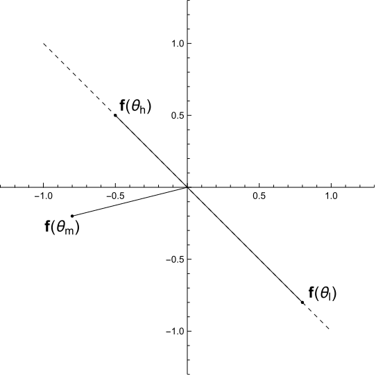
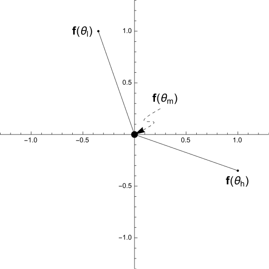
It turns out that for all linear combinations of two single-crossing functions and to be single crossing, Condition (4) of ratio ordering is required; see the proof of Lemma 1. Figure 4 illustrates: in panel 1(a), while ; in panel 1(b), and while . So in both cases, and are each single crossing but is not.
B.2 Proof of Lemma 1
When , the proof is trivial as all functions are single crossing and every pair of functions are ratio ordered. Hereafter, we assume .
It is clear that each function and is single crossing. We must show that and are ratio ordered.
First, let . Then , and . Thus, is single crossing from below and .
Second, let . Then and . Thus, is single crossing from above and .
Let . It follows that
Therefore, is not single crossing, a contradiction.
To prove (4), take any .
First, we show that implies and . Assume is not a zero function on , as otherwise the proof is trivial. Since is single crossing, either or . We consider the case of (and omit the proof for the other case, as it is analogous). Let . Since is single crossing and for , it holds that . It follows immediately that . As and are linearly dependent and is a non-zero vector, there exists such that for . Thus,
Next, we show that if and , then . Let . It follows that
As is single crossing, it follows that , as we wanted to show.
Assume that and are each single crossing. We prove the result for the case in which ratio dominates ; the other case is analogous. For any , we prove that is single crossing. We may assume that , as the result is trivial otherwise.
Suppose, towards contradiction, that is not single crossing. Claim 5 implies there exist such that either
| (16) | |||
| (17) |
First, we consider the case in which for all are non-zero vectors. Take any such that . As ratio dominates , by Condition (3), moves to in a clockwise rotation with an angle less than or equal to 180 degrees. Let be the clockwise angle from to . The vector defines a partition of into , , and . In both cases (16) and (17), both and are not in the same part of the partition that belongs to. Thus, and . On the other hand, both and are in the same closed half-space, either or , and is in the other closed half-space, either or , respectively. Thus, . Since Condition (3) implies , it follows that . Hence, and are linearly independent (), and similarly for and . However, and are linearly dependent (). This contradicts (4).
Second, suppose either or . We provide the argument assuming ; it is analogous if . Under either (16) or (17), . By Condition (4), and are linearly dependent. In particular, because , there exists a unique such that . Under either (16) or (17), , which contradicts the hypothesis that and are single crossing.
B.3 Proof of Proposition 2
The result is trivial if and it is equivalent to Lemma 1 if , so we may assume . The proof is also straightforward if all functions are multiples of one function , i.e., if there is such that . Thus, we further assume there exist such that and are linearly independent.
Assume and are (i) each single crossing and (ii) ratio ordered, and that there are functions such that . Then, for any function with finite support,
which is single crossing in by Lemma 1.
Take any such that and are linearly independent. Then, by Lemma 1, and are each single crossing and ratio ordered, as their linear combinations are all single crossing.
For every , let
We first prove the following claim:
Claim 7.
There exists such that .
-
Proof of Claim 7.
As and are linearly independent, there exists such that . Let . Then, for some , and .
The proof is complete if or . If not, take a lower and upper bound, and , of . Then . For otherwise, there exists such that . As and are between and , and is single crossing, we have , which contradicts . ∎
Now take any , the function , and in Claim 7. As , the system
| (18) |
has a unique solution . We will show that .
Suppose, towards contradiction, there exists such that
| (19) |
Let and respectively be a lower and an upper bound of . If , there is such that for . As is single crossing, we have for , which contradicts .454545The function must be single crossing because we can consider such that , , and for any . We use similar reasoning subsequently.
B.4 Proof of Theorem 2’s SCD⋆ Characterization
Here we only prove Theorem 2’s characterization of SCD⋆. The proof for its SSCD⋆ characterization is deferred to Supplementary Appendix SA.2.
Suppose that with each single crossing and ratio ordered. Then, for any , , which is single crossing by Lemma 1.
Assume, without loss of generality, that . Take any , and define . Define as , which, for every , is single crossing in .
We will show that, for every function with finite support, can be represented as a multiple of the difference between two convex utility combinations and . Since the environment is convex, there exist such that and for all . Since the utility difference is single crossing, so is . The result then follows from Proposition 2.
For any function with finite support, we define a function as an extension of :
In a sense, we let absorb the function values on . In particular, note that
We construct the Hahn-Jordan decomposition of . That is, we define functions by and . These are both functions with finite support, and . Let . If , pick an arbitrary with finite support and let . If , define with probability mass functions such that for any ,
Note that and have finite support. Since the environment is convex, there exist such that and for all . It follows that
which is single crossing.
Thus, if has SCD⋆, then is linear combinations SC-preserving. By Proposition 2, there exist and such that (i) and are each single crossing and ratio ordered, and (ii) . Hence, there exist functions with such that , or equivalently,
B.5 Proof of Proposition 1
We prove Proposition 1’s result about SCD⋆ and omit an analogous proof for the result about SSCD⋆. If , then the proof is trivial, so assume . The “if” direction of the result follows directly from Theorem 2: if has a positive affine transformation of the form in Proposition 1, then , as a positive affine transformation of , has SCD⋆.
For the “only if” direction, take any that has SCD⋆. Following the form given in Theorem 2, a positive affine transformation of is
where are each single crossing and ratio ordered.
First, we consider the case in which and are linearly dependent.464646This case can be ignored in the proof for SSCD⋆, because if and are strictly ratio ordered, then and must be linearly independent. Assume, with a positive affine transformation of , that the length of the vector in is either or for every . If , then because and are each single crossing, we have and . We can easily now rewrite in the form (6), with increasing.
Suppose ; we omit the analogous proof for the case of . By Condition (4) of ratio ordering, for every , the vector is linearly dependent on . As , there exists such that . Note that is increasing because and are each single crossing. If either (and so ) or (and so ), then
with the last term equal to zero. If, on the other hand, , then
Next, suppose that the vectors are linearly independent, so the angle between the vectors is strictly less than 180 degrees. As and are ratio ordered, for each there exists such that
or equivalently,
By Condition (4), , which implies that . A positive affine transformation of dividing by results in the form (6), where .
To prove that the function is increasing, take such that . To reduce notation below, let and for . We must show that , or equivalently that . Suppose ratio dominates ; the other case is analogous. Then , and hence
or equivalently,
Note that because ratio dominates , and and are linearly independent. Hence, .
Appendix C Proofs for MD⋆
The proof of Theorem 3 requires analogs of Lemma 1 and Proposition 2 for monotonic functions; these results are stated next but their proofs are deferred to Supplementary Appendix SA.4.
C.1 Aggregating Monotonic Functions
Lemma 2.
Let be monotonic functions. The linear combination is monotonic if and only if either or is an affine transformation of the other, i.e., there exists such that either or .
We say that is linear combinations monotonicity-preserving if is a monotonic function of for every function with finite support.
Proposition 3.
Let for some set . The function is linear combinations monotonicity-preserving if and only if there exist and such that (i) is monotonic, and (ii) .
C.2 Proof of Theorem 3
We omit the proof as it is similar to the proof of Theorem 2 in Appendix B.4.
The proof is trivial if , so assume there exists such that is not a zero function. Define by . Note that is a monotonic function of .
Let . As in the proof of Theorem 2 in Appendix B.4, for every with finite support, there exist convex utility combinations and , where and have finite support, such that is monotonic if and only if is monotonic. Since the environment is convex, the latter utility difference is indeed monotonic, and so is monotonic. By Proposition 3, there exist and such that . Hence, there exist functions with such that , or equivalently,
References
- One-switch independence for multiattribute utility functions. Operations Research 59 (3), pp. 764–771. Cited by: §1.3, §3.2.1, footnote 21, footnote 28.
- Sequential veto bargaining with incomplete information. Note: unpublished Cited by: §3.2.1.
- The theory of optimal delegation with an application to tariff caps. Econometrica 81 (4), pp. 1541–1599. Cited by: §1.1, §3.2.1.
- Monotone comparative statics under uncertainty. Quarterly Journal of Economics 117 (1), pp. 187–223. External Links: Document Cited by: §1.3, §6.
- A simple model of herd behavior. The Quarterly Journal of Economics 107 (3), pp. 797–817. Cited by: §4.2.
- A social choice lemma on voting over lotteries with applications to a class of dynamic games. Social Choice and Welfare 26 (2), pp. 285–304. External Links: Link Cited by: §3.2.1.
- Information design: a unified perspective. Journal of Economic Literature 57 (1), pp. 1–57. Cited by: Example 4.
- A theory of fads, fashion, custom, and cultural change as informational cascades. Journal of Political Economy 100 (5), pp. 992–1026. Cited by: §4.2.
- Noisy talk. Theoretical Economics 2 (4), pp. 395–440. Cited by: §4.1.
- When are local incentive constraints sufficient?. Econometrica 80 (2), pp. 661–686. External Links: ISSN 00129682, 14680262, Link Cited by: footnote 43.
- Implementation by gradual revelation. RAND Journal of Economics 46 (2), pp. 271–296. External Links: Document, Link Cited by: §1.3, §3.2.1.
- Strategic information transmission. Econometrica 50 (6), pp. 1431–1451. Cited by: §1.1, §4.1, §4.1, §4.1, footnote 34.
- On the intuition of rank-dependent utility. Journal of Risk and Uncertainty 23 (3), pp. 281–298. External Links: Link Cited by: Example 2.
- Majority voting over lotteries: conditions for existence of a decisive voter. Economics Bulletin 34 (1), pp. 263–270. Cited by: §1.3, §3.2.1, footnote 41.
- Von neumann-morgenstern utility functions on two attributes. Operations Research 22 (1), pp. 35–45. Cited by: §1.3.
- Majority voting with single-crossing preferences. Journal of Public Economics 59 (2), pp. 219–237. External Links: Document Cited by: §4.3.
- Cardinal welfare, individualistic ethics, and interpersonal comparisons of utility. Journal of Political Economy 63 (4), pp. 309–321. Cited by: footnote 25.
- Collective dynamic choice: the necessity of time inconsistency. American Economic Journal: Microeconomics 7 (4), pp. 150–78. External Links: Document, Link Cited by: footnote 25.
- Semicontinuous extension of a partial order. Journal of Mathematical Economics 2 (3), pp. 395–406. External Links: Document, Link Cited by: footnote 10.
- Bayesian persuasion. American Economic Review 101 (6), pp. 2590–2615. Cited by: Example 4.
- Total positivity. Vol. I, Stanford University Press, Stanford, California. Cited by: §1.3, §3.3, footnote 29.
- Beyond unbounded beliefs: how preferences and information interplay in social learning. Note: unpublished Cited by: §4.2.
- Single-crossing differences on distributions. Note: unpublished Cited by: §4, footnote 29, footnote 41, footnote 6.
- Optimal delegation in a multidimensional world. Note: unpublished Cited by: §3.2.1.
- On the equivalence of bayesian and dominant strategy implementation for environments with nonlinear utilities. Economic Theory 67 (3), pp. 617–644. Cited by: §1.3, §5.1.
- Communication in settings with no transfers. RAND Journal of Economics 22 (2), pp. 173–198. Cited by: §4.1, §4.1, footnote 34.
- Good news and bad news: representation theorems and applications. Bell Journal of Economics 12 (2), pp. 380–391. Cited by: footnote 12.
- Putting auction theory to work. Cambridge University Press. Cited by: §2.
- Monotone comparative statics. Econometrica 62 (1), pp. 157–180. Cited by: §A.2, §1.1, §1.1, §1.3, §2, §5.2, §5.2, §5.2, footnote 44.
- Real analysis with economic applications. Vol. 10, Princeton University Press. Cited by: footnote 10.
- Aggregating the single crossing property. Econometrica 80 (5), pp. 2333–2348. Cited by: §1.3, §3.3.
- A theory of anticipated utility. Journal of Economic Behavior & Organization 3 (4), pp. 323–343. External Links: Document, Link Cited by: §1.1, Example 2.
- Order restricted preferences and majority rule. Social Choice and Welfare 7 (4), pp. 331–342. External Links: Link Cited by: §1.1, §2, §4.3.
- Effective cheap talk with conflicting interests. Journal of Economic Theory 50 (2), pp. 445–458. Cited by: §4.1.
- The strategy of ambiguity: uncertainty and electoral competition. American Political Science Review 66 (2), pp. 555–568. Cited by: §1.1, §4.3.
- Frictional matching models. Annual Review of Economics 3 (1), pp. 319–338. External Links: Document, https://doi.org/10.1146/annurev-economics-111809-125046, Link Cited by: footnote 5.
- Minimizing a submodular function on a lattice. Operations Research 26 (2), pp. 305–321. Cited by: §1.3.
- Majority rule with lotteries on alternatives. Quarterly Journal of Economics 83 (4), pp. 696–703. Cited by: §1.1, §4.3.