Delegation in Veto Bargaining

A proposer requires the approval of a veto player to change a status quo. Preferences are single peaked. Proposer is uncertain about Vetoer’s ideal point. We study Proposer’s optimal mechanism without transfers. Vetoer is given a menu, or a delegation set, to choose from. The optimal delegation set balances the extent of Proposer’s compromise with the risk of a veto. Under reasonable conditions, “full delegation” is optimal: Vetoer can choose any action between the status quo and Proposer’s ideal action. This outcome largely nullifies Proposer’s bargaining power; Vetoer frequently obtains her ideal point, and there is Pareto efficiency despite asymmetric information. More generally, we identify when “interval delegation” is optimal. Optimal interval delegation can be a Pareto improvement over cheap talk. We derive comparative statics. Vetoer receives less discretion when preferences are more likely to be aligned, by contrast to expertise-based delegation. Methodologically, our analysis handles stochastic mechanisms.

1 Introduction

Motivation.

There are numerous situations in which one agent or group can make proposals but another must approve them. Legislatures (e.g., the U.S. Congress) send bills to executives (e.g., the President), who can veto them. Governmental legislation can be struck down as unconstitutional by the judiciary. Prosecutors choose which charges to bring against defendants, but judges and juries decide whether to convict. A real-estate agent can recommend a house to his client, but the client must decide to put in an offer; similarly, a search committee can put forward a candidate, but the organization decides whether to hire her.

Romer and Rosenthal (1978) present a seminal analysis of such veto bargaining. Their framework is one of complete information in which a proposer (Congress, government, prosecutor, salesperson, search committee) makes a take-it-or-leave-it proposal to a veto player (President, judiciary, judge/jury, customer, organization). Preferences are single peaked. That is, rather than “dividing a dollar”, the negotiating parties share some preference alignment. Such preferences are plausible in the contexts mentioned above.

Our paper studies veto bargaining with incomplete information. The proposer is uncertain about the veto player’s preferences—specifically, which proposals would actually get vetoed. Previous scholars have emphasized this feature’s importance; see Cameron and McCarty’s (2004) survey. But to our knowledge, our paper is the first that takes a general approach to the issue. We do not assume the proposer is restricted to making a single proposal (e.g., Romer and Rosenthal, 1979), nor do we fix any particular negotiating protocol (e.g., one round of cheap talk in Matthews, 1989; Forges and Renault, 2021). Instead, we consider the possible outcomes across all possible protocols by taking a mechanism design approach. Our focus is on identifying the proposer’s optimum.

There are at least two reasons this mechanism design approach is of interest. First, it identifies an upper bound on the proposer’s welfare. Second, as is standard in settings without transfers, any (deterministic) mechanism is readily interpreted and implemented as delegation. That is, the proposer simply offers a menu of options; the veto player can select any one or reject them all. Menus or delegation sets are observed in practice in some applications of our model. Salespeople show customers subsets of products, and search committees put forward multiple candidates for their organization to choose among. In politics, a bill authorizing at most $$x$ of spending effectively offers an executive who controls the implementing bureaucracy the choice of any spending level in the interval $[0,x]$. Bills can also grant more or less discretion of how to allocate a given level of spending, as encapsulated by former Senator Russ Feingold in the context of the first U.S. coronavirus stimulus package: “Congress has to decide how much discretion it wants to delegate to executive branch officials.” (Washington Post, March 22, 2020.)

Main results.

We formally study a one-dimensional environment. There is a status quo policy or action, $0$, that obtains if there is a veto. There are two agents. Proposer’s ideal action is $1$. Vetoer’s ideal action, $v$, is her private information. We assume Vetoer preferences are represented by a quadratic loss function, but allow Proposer to have any concave utility function.

Our first result (Proposition 1) identifies conditions under which it is optimal for Proposer to fully compromise and simply let Vetoer choose her preferred action in the interval $[0,1]$. We call this full delegation, because Proposer only excludes options that are, from his point of view, dominated by simply offering his ideal action $1$ no matter Vetoer’s ideal point. Intuitively, full delegation is optimal when the specter of a veto looms large; in particular, it is sufficient that the density of Vetoer’s ideal point is decreasing on the unit interval. Optimality of full delegation is quite striking: despite Proposer having considerable bargaining and commitment power, it is Vetoer who frequently gets her first best. This is a telling manifestation of private information’s consequences. Since full delegation implies ex-post Pareto efficiency, large information rents can obtain here without generating inefficiency, unlike in most other settings.

The opposite of full delegation is no compromise: Proposer only offers his ideal action, $1$. Of course, Vetoer can veto and choose the status quo $0$. Proposition 2 gives conditions for optimality of no compromise. It is sufficient, for example, that Proposer has a linear loss function—so, in the relevant region of actions, $[0,1]$, he only cares about the mean action—and the density of Vetoer’s ideal point is increasing in this region. This case juxtaposes nicely against the aforementioned decreasing-density condition for full delegation.

Both full delegation and no compromise are boundary cases of interval delegation: Proposer offers a menu of the form $[c,1]$. Interval delegation is interesting for multiple reasons. Among them are that such delegation sets are simple to interpret and implement, and they turn out to be tractable for comparative statics. Proposition 3 provides conditions under which interval delegation is optimal. These are met, in particular, when Proposer has a linear or quadratic loss function and Vetoer’s ideal point distribution is logconcave (Corollary 3).

We show that, under reasonable conditions, optimal interval delegation yields a Pareto improvement over singleton proposals, even when cheap talk is allowed and full delegation is not optimal (Proposition 5). We trace the intuition to Proposer being more willing to compromise when he can offer Vetoer an interval of options rather than only singletons.

We develop two comparative statics, restricting attention to interval delegation — either justified by optimality or otherwise. First, what happens when Proposer becomes more risk averse? Proposition 4(i) establishes that Vetoer is given more discretion: the optimal threshold in the interval delegation set (i.e., that denoted $c$ above) decreases. Intuitively, Proposer offers a larger set of options to mitigate the risk of a veto. Second, what about when Vetoer becomes more ex-ante aligned with Proposer? Formally, we consider right shifts in Vetoer’s ideal point distribution, in the sense of likelihood ratio dominance. Proposition 4(ii) establishes that discretion decreases: the optimal interval delegation threshold increases. Intuitively, this is because Proposer is less concerned that a veto will occur. Although these comparative statics appear natural, it is the structure of interval delegation that allows us to establish them.

Contrast with expertise-based delegation.

The second comparative static mentioned above contrasts with a key theme of the expertise-based delegation literature following Holmström (1977, 1984). In that literature, an agent is given discretion over actions because her private information is valuable to the principal; the principal limits the degree of discretion because of preference misalignment. One version of the so-called Ally Principle says that a more aligned agent receives more discretion. Holmström (1984) establishes its validity under reasonably general conditions, so long as delegation sets take the form of intervals. In our setting, the reason Proposer gives Vetoer discretion is fundamentally different from that in Holmström: it is not to benefit from Vetoer’s expertise; rather, Proposer trades off the risk of a veto with the extent of compromise. (In jargon, our delegator has state-independent preferences, by contrast to the state-dependent preferences in most of the literature following Holmström.) Hence we find less discretion emerging when there is, in a suitable sense, more ex-ante preference alignment.

Applications.

In Section 5 we present three applications: product menus offered to a consumer; the legal doctrine of lesser-included offenses; and legislative bills put forward to an executive. These applications illustrate the relevance of our general results and allow us to discuss additional implications. For example, we comment on voluntary disclosure of information by consumers to sellers; welfare consequences of the lesser-included offenses doctrine; and alternative interpretations of how discretion can be granted in the legislative application.

Methodology.

We hope some readers will find our analysis interesting on a methodological level. While it is convenient and economically insightful to describe our substantive results in terms of optimal delegation sets, the formal problem we study is one of mechanism design without transfers. Our analytical methodology builds on the infinite-dimensional Lagrangian approach advanced by Amador et al. (2006) and Amador and Bagwell (2013). Unlike these authors and many others, including the important contributions by Melumad and Shibano (1991) and Alonso and Matouschek (2008), we also cover stochastic mechanisms. That is, we allow for mechanisms in which Vetoer may choose among lotteries over actions. We view such mechanisms as not only theoretically important, but also relevant in applications. For instance, consider a President (Proposer) nominating a judge for confirmation from the Senate (Vetoer) to a lifetime appointment. Both the President and the (pivotal voter in the) Senate have preferences over the ideology of the appointed judge. While some potential nominees have extensive written records or well-identified ideologies, others have less of a record of their own legal opinions and thus could be viewed as a lottery over ideologies.

Stochastic mechanisms can sometimes be optimal in our framework. Nevertheless, we establish that our sufficient conditions for full delegation, no compromise, and interval delegation (Propositions 1, 2, and 3) ensure optimality of these (deterministic) mechanisms even among stochastic mechanisms. Furthermore, by permitting stochastic mechanisms, our sufficient conditions are shown to also be necessary for a class of Proposer’s utility functions that include linear and quadratic loss. Our approach to handling stochastic mechanisms should be useful in other delegation problems.

Recently, Kolotilin and Zapechelnyuk (2019) have introduced balanced delegation problems, which are delegation problems in which certain extreme actions or outside options must be included. Our setting fits into their general framework, as one can assume the status quo must be part of the delegation set. Kolotilin and Zapechelnyuk derive a general equivalence between such problems and monotone Bayesian persuasion problems. More concretely, they show how some results from the latter literature (e.g., Kolotilin, 2018; Dworczak and Martini, 2019) can be brought to bear on “linear” balanced delegation problems. Our approach of directly studying the delegation problem is complementary and has some advantages. First, it permits insights absent said linearity: this is most evident in our full delegation result. Second, we believe it provides some more transparent economic intuitions. Third, unlike Kolotilin and Zapechelnyuk (2019), we can address stochastic mechanisms and necessity of our sufficient conditions. At a broader level, note that by contrast to us, Kolotilin and Zapechelnyuk (2019) highlight applications concerning expertise-based delegation (i.e., with state-dependent delegator preferences). Zapechelnyuk (2019) applies their methodology to a quality certification problem that, he shows, maps into a delegation problem in which the delegator’s preferences are state independent.

Like us, Saran (2020) and Amador and Bagwell (2021) directly analyze delegation problems with an outside option. Iterations of both papers have developed concurrently with ours. Both papers study frameworks that are more general than ours insofar as they allow for state-dependent delegator preferences. Our approach to finding conditions for the optimality of delegation sets differs from theirs. This is most evident in that neither Saran (2020) nor Amador and Bagwell (2021) consider stochastic mechanisms or necessity of their sufficient conditions. Our approach also allows us to deduce more permissive sufficient conditions for our delegation sets than their results would when specialized to state-independent delegator preferences. Furthermore, our comparative statics and comparisons with cheap talk are distinct.

Outline.

The rest of the paper proceeds as follows. Section 2 presents our model. Section 3 contains our main results on the conditions for optimality of full delegation, no compromise, and, more broadly, interval delegation. Section 4 develops comparative statics and makes comparisons with other mechanisms. Section 5 contains our applications. Section 6 concludes. All proofs are in the appendices.

2 Model

2.1 Veto Bargaining with Incomplete Information

We consider a classic bargaining problem between two players, a proposer (he) and a veto player (she), who jointly determine a policy outcome or action $a\in ℝ$. In a manner elaborated below, Proposer makes a proposal that Vetoer can either accept or reject. If Vetoer rejects, a status-quo action is preserved; we normalize the status quo to $0$.

We assume both players have single-peaked utilities. Proposer’s utility is $u(a)$ that is concave, maximized uniquely at $a=1$ (essentially a normalization), and twice differentiable at all $a\ne 1$. Unless indicated explicitly, we use ‘concave’, ‘increasing’, ‘negative’, etc., to mean ‘weakly concave’, ‘weakly increasing’, ‘weakly negative’, etc. We will sometimes invoke a restriction to the following subclass of Proposer preferences, which stipulates a convex combination of the widely-used linear and quadratic loss functions.

Condition LQ.

For some $\gamma \in [0,1]$,

$$u(a)=-(1-\gamma )|1-a|-\gamma {(1-a)}^2.$$

Vetoer’s utility is represented by $-l(|v-a|)$, where $l(\cdot )$ is strictly increasing. So her utility is symmetric around the unique ideal point $v$. For tractability, we assume $l(|v-a|)={(v-a)}^2$. A subset of our results will rely only on Vetoer’s ordinal preferences, for which the choice of quadratic loss entails no loss of generality given that Vetoer’s utility is symmetric around her ideal point. Specifically, Vetoer’s ordinal preferences are sufficient when we consider only deterministic mechanisms.

A key ingredient of our model is that $v$ is Vetoer’s private information. We accordingly refer to $v$ as Vetoer’s type. It is drawn from a cumulative distribution $F$ whose support is an interval $[\underset{¯}{v},\overline{v}]$, where we permit $\underset{¯}{v}=-\mathrm{\infty }$ and/or $\overline{v}=\mathrm{\infty }$. We assume $F$ admits a continuously differentiable density $f$, and that $f(\cdot )>0$ on $[0,1]$. All aspects of the environment except the type $v$ are common knowledge. If $v$ were common knowledge, this model would reduce to that of Romer and Rosenthal (1978).

Naturally, it is in Proposer’s interests to elicit information from Vetoer about $v$. For example, they might engage in cheap talk communication (Matthews, 1989), possibly over multiple rounds, or Proposer might make sequential proposals, and so on. To circumvent issues about exactly how the bargaining ensues, we take a mechanism design approach. Following the revelation principle, we consider direct revelation mechanisms, hereafter simply mechanisms.

A deterministic mechanism is described by a real-valued function $\alpha (v)$, which specifies the action when Vetoer’s type is $v$, and must satisfy the usual incentive compatibility (IC) and individual rationality (IR) conditions. IC requires that each type $v$ prefers $\alpha (v)$ to $\alpha (v^{\prime })$ for any $v^{\prime }\ne v$; IR requires that each type $v$ prefers $\alpha (v)$ to the status quo $0$. Notice that any deterministic mechanism is equivalent to the Proposer offering a (closed) menu or delegation set $A\subseteq ℝ$, and Vetoer choosing an action from $A\cup \{0\}$. We will also consider the more general class of stochastic mechanisms, which specify probability distributions over actions for each Vetoer type, with analogous IC and IR constraints to those aforementioned. Stochastic mechanisms are theoretically important because the revelation principle does not justify focusing only on deterministic mechanisms. As noted in the introduction, they may also be relevant for applications. A notable contribution of this paper is to establish conditions under which, despite the absence of transfers, stochastic mechanisms cannot improve upon deterministic ones.

The mechanism design approach we take can be viewed as identifying an upper bound on Proposer’s welfare. That said, as also mentioned in the introduction, we find the implementation via delegation sets quite realistic in various contexts.

2.2 Proposer’s Problem

We now formally define Proposer’s problem. Let $M(ℝ)$ denote the set of Borel probability distributions on $ℝ$, and $M_0(ℝ)$ be the subset of distributions with finite expectation and finite variance. Denote by ${\delta }_a$ the degenerate distribution that puts probability 1 on action $a$. A stochastic mechanism—or simply a mechanism without qualification—is a measurable function $m:[\underset{¯}{v},\overline{v}]\to M_0(ℝ)$, with $m(v)$ being the probability distribution over actions for type $v$. To reduce notation, for any deterministic mechanism $\alpha :[\underset{¯}{v},\overline{v}]\to ℝ$, we also denote the mechanism $v\mapsto {\delta }_{\alpha (v)}$ by $\alpha$. For any integrable function $g:A\to ℝ$, let ${𝔼}_{m(v)}[g(a)]$ denote the expectation of $g(a)$ when $a$ has distribution $m(v)$. We only consider mechanisms $m$ for which $v\mapsto {𝔼}_{m(v)}[a]$ is integrable. Define the subset of mechanisms

That is, $𝒮$ consists of mechanisms in which type $0$ gets the status quo and a higher type receives a higher expected action. The first requirement is implied by IR, since Vetoer can always choose the status quo. The second is implied by IC, since Vetoer’s utility $-{(v-a)}^2$ is equivalently represented by $av-a^2/2$; singlecrossing difference in $(a,v)$ yields monotonicity of ${𝔼}_{m(v)}[a]$ in $v$ from standard arguments (elaborated in fn. 14 below).

Proposer’s problem is:

$\underset{m\in 𝒮}{\max }{\displaystyle \int {𝔼}_{m(v)}[u(a)]dF(v)}$ (P)

$\text{s.t. }{𝔼}_{m(v)}\left[av-a^2/2\right]={\displaystyle {\int }_0^v}{𝔼}_{m(s)}[a]ds\forall v\in [\underset{¯}{v},\overline{v}].$ (IC-env)

As noted above, it is without loss to restrict attention to mechanisms in $𝒮$. The constraint (IC-env) captures the additional content of IC, beyond monotonicity, via an analog of the standard envelope formula. Note that since IC requires that no type prefer type $0$’s lottery over its own, and type $0$’s IR constraint requires that it receive action $0$ (captured in $𝒮$), every type’s IR constraint is implied by type $0$’s. An optimal mechanism is a solution to problem (P).

If we restricted attention to deterministic mechanisms, the analogous problem for Proposer would be:

$\underset{\alpha \in 𝒜}{\max }{\displaystyle \int u(\alpha (v))dF(v)}$ (D)

$\text{s.t. }v\alpha (v)-\alpha {(v)}^2/2={\displaystyle {\int }_0^v}\alpha (s)ds,$

where

$$𝒜:=\{\alpha :[\underset{¯}{v},\overline{v}]\to ℝ|\alpha (0)=0\text{ and }\alpha \text{ is increasing}\}.$$

Any deterministic mechanism $\alpha$ that is IC has a corresponding (closed) delegation set $A_{\alpha }:={\bigcup }_v\alpha (v)$. Conversely, any delegation set $A$ has a corresponding deterministic mechanism ${\alpha }_A$ where ${\alpha }_A(v)$ is the action in $A\cup \{0\}$ that type $v$ prefers the most (with ties broken in favor of Proposer). Note that ${\alpha }_A$ satisfies IC and IR. While our formal analysis works with mechanisms, it is easier and more economically intuitive to describe our main results, which concern certain deterministic mechanisms, using delegation sets.

We emphasize some terminology: an optimal deterministic mechanism (or an optimal delegation set) is a solution to problem (D). But when we say that a deterministic mechanism (or delegation set) is optimal, we mean that it solves problem (P), i.e., no stochastic mechanism can strictly improve on it.

2.3 Discussion

Let us comment on four aspects of our model.

First, veto power is captured via a standard interim IR constraint. An alternative, as in Compte and Jehiel (2009), would be to allow Vetoer to exercise her veto even after the mechanism determines an action. This is stronger than just ex-post IR because it also strengthens the IC constraint: when type $v$ mimics type $v^{\prime }$, $v$ may veto a different set of allocations than $v^{\prime }$ would, and so the action distribution that $v$ evaluates the deviation with is not $m(v^{\prime })$. Which form of veto power is conceptually appropriate depends on the application. But any IC and IR deterministic mechanism also satisfies the ex-post veto constraint. Hence, the sufficient conditions we provide below for optimality of delegation sets would remain sufficient.

Second, our model is one of private values: Vetoer’s type does not affect Proposer’s preferences. This is by way of contrast with the delegation literature initiated by Holmström (1984), in which a principal gives discretion to an agent because of the agent’s expertise, i.e., because they have interdependent preferences. We could extend our model and analysis to incorporate this expertise-based delegation or discretion aspect, but one of our main themes is that discretion will emerge even when that is absent, because we instead have veto power.

Third, one might ask why Vetoer relies on Proposer in the first place given private values. Why can’t the Vetoer simply choose her ideal point, or require Proposer to offer all the options? At a formal level, we simply take the veto bargaining institution and Proposer’s agenda setting power as given, for reasons outside the model. But it is plausible in many situations that even though Vetoer knows her preferences, she nevertheless relies on Proposer to provide the options. In the hiring application mentioned earlier, a superior within an organization may well know her preferences, but lacks the time or expertise to find candidates herself. She thus relies on the search committee. In an application elaborated on in Delegation in Veto Bargaining, a consumer cannot pick among products a salesperson chooses not to make available (and the salesperson can always claim some products are out of stock). A related point in the legislative context is that even when Vetoer knows her spatial/ideological preferences, she cannot simply implement her preferred policy: implementation must be preceded by policy development, which is done by Proposer (cf.  Hirsch and Shotts, 2015).

Fourth, while we have assumed that Proposer has an ideal point of $1$, an equivalent formulation is that Proposer’s utility $u(a)$ is globally increasing but he is constrained to only offer actions less than $1$, or there is simply an upper bound on the action space at $1$.

2.4 Preliminary Observations

Consider delegation sets. Notice first that there is no loss for Proposer in including his ideal action $1$ in the delegation set: for any Vetoer type $v$, either it does not affect the chosen action, or it results in a preferable action. Next, there is no loss for Proposer in excluding actions outside $[0,1]$: shrinking a delegation set $A$ that contains $1$ to $A\cap [0,1]$ only results in each type choosing an action closer to $1$. As existence of an optimal delegation set follows from standard arguments, we have:

Lemma 1.

There is an optimal delegation set $A$ satisfying $1\in A\subseteq [0,1]$.

It would also be without loss to assume that a delegation set contains the status quo, $0$. We don’t do so, however, because it is convenient to sometimes describe optimal delegation sets without including $0$.

For any $a\in (0,1)$, the delegation set $A=[a,1]$ strictly dominates the singleton $\{a\}$ because $A$ results in preferable actions for Proposer when $v>a$. This simple observation highlights the significance of giving Vetoer discretion, despite our model shutting down the expertise-based rationale that the literature initiated by Holmström (1984) has focused on.

While Proposer always wants to include action $1$ in the delegation set, he faces a tradeoff when including any action $a\in (0,1)$. Allowing Vetoer to choose such an action $a$ reduces the probability of a veto (or any action less than $a$) but also reduces the probability that Vetoer chooses an action even higher than $a$, which Proposer would prefer to $a$.

3 Delegation and Optimal Mechanisms

3.1 Full Delegation

In light of Lemma 1, we refer to the delegation set $[0,1]$ as full delegation. Note that full delegation does impose some constraints on Vetoer. But the constraints are minimal: only actions outside the convex hull of the status quo and Proposer’s ideal point are excluded. Given the veto-bargaining institution, an outcome of full delegation starkly captures how Vetoer’s private information can corrode Proposer’s bargaining or agenda-setting power. All Vetoer types in $[0,1]$ obtain their ideal action; no matter Vetoer’s type, there is (ex-post) Pareto efficiency, unlike in most other settings that confer information rents. Full delegation thus contrasts sharply with the outcome under complete information (Romer and Rosenthal, 1978), in which case Proposer would make Vetoer with ideal point indifferent with exercising the veto while getting his own ideal action $1$ from types $v\ge 1/2$. It also contrasts with the outcome under incomplete information were Proposer restricted to making a singleton proposal. In that case the proposal would lead to a veto by some subinterval of types $v\in [0,1]$, hence to ex-post Pareto inefficiency, and all Vetoer types would be weakly worse off, many strictly.

It is thus of interest to know when full delegation is optimal. The following quantity concerning the concavity of Proposer’s utility will play a key role in our analysis:

$$\kappa :=\underset{a\in [0,1)}{inf}-u^{\prime \prime }(a).$$

Under Condition LQ, $\kappa =2\gamma$, which is larger when Proposer’s utility puts more weight on its quadratic component relative to its linear component.

Proposition 1 (Full delegation).

Full delegation is optimal if

$$\kappa F(v)-u^{\prime }(v)f(v)\text{ is increasing on }[0,1].$$ (1)

Conversely, under Condition LQ, full delegation is optimal only if (1) holds.

Since $\kappa \ge 0$, $F(\cdot )$ is increasing, and $u^{\prime }(\cdot )$ is decreasing and nonnegative on $[0,1]$, the proposition directly implies:

Corollary 1.

Full delegation is optimal if the type density is decreasing on $[0,1]$.

In particular, it is sufficient for full delegation that the type distribution is unimodal with a negative mode. To obtain intuition for the corollary, consider removing any interval $(\underset{¯}{a},\overline{a})$ from a delegation set $A$ that contains $[\underset{¯}{a},\overline{a}]$. This change induces Vetoer with type $v\in (\underset{¯}{a},\overline{a})$ to choose between $\underset{¯}{a}$ and $\overline{a}$. Due to her symmetric utility function, Vetoer will choose $\underset{¯}{a}$ when $v\in (\underset{¯}{a},\frac{\underset{¯}{a}+\overline{a}}{2})$, which harms Proposer, while Vetoer will choose $\overline{a}$ when $v\in (\frac{\underset{¯}{a}+\overline{a}}{2},\overline{a})$, which benefits Proposer. When the type density is decreasing on $[\underset{¯}{a},\overline{a}]$, the former possibility is more likely. In fact, the pruned delegation set induces an action distribution that is second-order stochastically dominated if the type density is decreasing on $[\underset{¯}{a},\overline{a}]$. Since Proposer’s utility is concave, he prefers the original delegation set $A$. As any (closed) delegation set contained in $[0,1]$ can be obtained by successively removing open intervals from $[0,1]$, full delegation is an optimal delegation set. While this explanation applies only among delegation sets, Proposition 1 implies that Corollary 1 holds even allowing for stochastic mechanisms.

Removing an interval increases the expected action when the type density is increasing, but it also increases the probability of a lower action. Thus, when Proposer is risk averse, it can be optimal to not remove an interval even if the density is increasing on that interval. This explains why condition (1) is weaker than $f$ decreasing on $[0,1]$. In general, removing an interval is optimal only if the density is increasing quickly relative to Proposer’s risk aversion. This suggests that full delegation is optimal whenever Proposer is sufficiently risk averse. Proposition 1 allows us to formalize the point using the Arrow-Prat (Arrow, 1965; Pratt, 1964) coefficient of absolute risk aversion.

Corollary 2.

Full delegation is optimal if Proposer is sufficiently risk averse, i.e., if $\underset{a\in [0,1)}{inf}-u^{\prime \prime }(a)/u^{\prime }(a)$ is sufficiently large.

It should be noted that (regardless of Proposer’s risk aversion) optimality of full delegation does require our maintained assumption of $\underset{¯}{v}\le 0$. Were Vetoer’s lowest type $\underset{¯}{v}\in (0,1)$, then full delegation—or even the interval $[\underset{¯}{v},1]$—would never be an optimal delegation set: it would be strictly worse than $[\min \{2\underset{¯}{v},1\},1]$.

Readers familiar with Alonso and Matouschek (2008) may find it helpful to draw a connection between that paper and our Proposition 1. If we had restricted attention to deterministic mechanisms and assumed that Proposer’s utility is a quadratic loss function, then the sufficiency result in Proposition 1 would follow from a result in Alonso and Matouschek (2008), even though their model does not have a veto constraint and, as such, highlights expertise-based delegation. To make the connection, we observe that when $u(a)=-{(1-a)}^2$, condition (1) is equivalent to Alonso and Matouschek’s “backward bias” (p. 264) being convex on $[0,1]$. Their Proposition 2 then implies that if $\{0,1\}$ is contained in the optimal delegation set, then the interval $[0,1]$ is contained in the optimal delegation set. But recall from Lemma 1 that in choosing among delegation sets, Proposer need not offer any action outside $[0,1]$ and can offer his ideal point $1$; moreover, he may as well offer the status quo $0$. It follows that full delegation is an optimal delegation set. We emphasize, therefore, that Proposition 1 establishes optimality among more general Proposer preferences and stochastic mechanisms.

Consider now necessity in Proposition 1. If Proposer has a linear loss utility, then our preceding discussion explains why a delegation set $A$ containing $[\underset{¯}{a},\overline{a}]\subseteq [0,1]$ should be pruned to $A\setminus (\underset{¯}{a},\overline{a})$ if the type density is increasing on this interval: the expected action increases. Hence, the converse of Corollary 1 holds for linear loss utility. For quadratic loss utility (and with additional smoothness assumptions), Alonso and Matouschek’s (2008) Proposition 2 implies that $f(v)$ need not be decreasing on $[0,1]$ for full delegation to be optimal, but a weaker condition is necessary: $F(v)-(1-v)f(v)$ must be increasing on $[0,1]$. Proposition 1 subsumes these two cases by deducing necessity of condition (1) for the linear-quadratic family of utilities (Condition LQ).

3.2 No Compromise

The other extreme from full delegation is no compromise: Proposer makes a take-it-or-leave-it offer of his own ideal action, not offering any other action. Of course, Vetoer can choose the status quo as well. When Proposer has a linear loss utility—or, a fortiori, if we had permitted $u(a)$ to be convex on $[0,1]$—then no compromise is an optimal delegation set whenever the type density $f$ is increasing on $[0,1]$. This follows from reversing the previous subsection’s second-order stochastic dominance argument for optimality of full delegation when $f$ is decreasing. But neither is linear loss utility nor convexity of $F$ on $[0,1]$ required for optimality of no compromise.

Proposition 2.

Assume Condition LQ. No compromise is optimal if and only if

$$(u^{\prime }(1)+\kappa (1-t))\frac{F(t)-F(1/2)}{t-1/2}\ge (u^{\prime }(0)-\kappa s)\frac{F(1/2)-F(s)}{1/2-s}\text{ for all }1\ge t>1/2>s\ge 0.$$

Under linear loss utility (so $u^{\prime }(1)=u^{\prime }(0)=1$ and $\kappa =0$), the condition in Proposition 2 simplifies to $f(1/2)$ being a subgradient of $F$ at $1/2$ on the domain $[0,1]$. This subgradient condition is weaker than $F$ being convex on $[0,1]$.

Remark 1.

With linear loss utility, no compromise can be an optimal delegation set (i.e., deterministic mechanism) even if the subgradient condition does not hold. However, there will then be a stochastic mechanism that Proposer strictly prefers. This situation can arise, for example, when the type density is strictly increasing except on a small interval around $1/2$, where it is strictly decreasing. Intuitively, Proposer would like to delegate a small set of actions around $1/2$ to types close to $1/2$, but adding such actions to the no-compromise delegation set is deleterious because it leads to many types above $1/2$ choosing an action close to $1/2$ rather than $1$. By contrast, lotteries with expected value $1/2$ can be used to attract only types close to $1/2$. Example E.1 in Appendix E elaborates. $\diamond$

Although Proposition 2 assumes Condition LQ, we note that no compromise can be an optimal delegation set even otherwise. In particular, it can be shown that if no compromise is an optimal delegation set for some $u$, then it is also an optimal delegation set for any utility function that is a convex transformation of $u$.

On the other hand, no compromise is not optimal—not even an optimal delegation set—if Proposer’s utility is differentiable at his ideal point $a=1$ (which implies $u^{\prime }(1)=0$). The reason is that when $u^{\prime }(1)=0$, Proposer would strictly benefit from offering a small interval $[1-\epsilon ,1]$, or even just the action $1-\epsilon$, instead of only offering action $1$. For, Proposer’s decrease in utility from getting an action slightly lower than $1$ is second order, but there is a first-order increase in the probability of avoiding a veto.

3.3 Interval Delegation

Both full delegation and no compromise are special cases of interval delegation: Proposer offers an interval, and Vetoer chooses an action from either that interval or the status quo. It follows from Lemma 1 that when interval delegation is optimal, there is always an optimal interval of the form $[c,1]$ for some $c\in [0,1]$. One can thus interpret interval delegation as Proposer designating a minimally acceptable option; implicitly, the maximal acceptable option is Proposer’s ideal point. Interval delegation, without a status quo, has been a central focus of the prior literature: intervals are simple, tractable, and lend themselves to comparative statics. Arguably, intervals also map more naturally into proposals likely to emerge in applications.

Proposition 3.

The interval delegation set $[c^{\ast },1]$ with $c^{\ast }\in [0,1]$ is optimal if

1. $\kappa F(v)-u^{\prime }(v)f(v)$ is increasing on $[c^{\ast },1]$;

2. $\left(u^{\prime }(c^{\ast })+\kappa (c^{\ast }-t)\right)\frac{F(t)-F(c^{\ast }/2)}{t-c^{\ast }/2}\ge u^{\prime }(c^{\ast })\frac{F(c^{\ast })-F(c^{\ast }/2)}{c^{\ast }/2}$ for all $t\in (c^{\ast }/2,c^{\ast }]$; and

3. $u^{\prime }(c^{\ast })\frac{F(c^{\ast })-F(c^{\ast }/2)}{c^{\ast }/2}\ge \left(u^{\prime }(0)-\kappa s\right)\frac{F(c^{\ast }/2)-F(s)}{c^{\ast }/2-s}$ for all $s\in [0,c^{\ast }/2)$.

Conversely, under Condition LQ, the delegation set $[c^{\ast },1]$ with $c^{\ast }\in (0,1)$ is optimal only if conditions (i), (ii), and (iii) above hold.

We discuss sufficiency. The intuition for condition (i) in the proposition is analogous to that discussed after Proposition 1; it ensures that there is no benefit to not fully delegating the interval $[c^{\ast },1]$ taking as given that Vetoer can choose $c^{\ast }$. For linear loss utility, the condition reduces to $F$ being concave on $[c^{\ast },1]$. Linear loss utility is also helpful to interpret the other conditions. Conditions (ii) and (iii) then simplify to the requirements that the average density from $c^{\ast }/2$ to $c^{\ast }$ be simultaneously less than that from $c^{\ast }/2$ to $t$ for all $t\in (c^{\ast }/2,c^{\ast }]$ and greater than that from $s$ to $c^{\ast }/2$ for all $s\in [0,c^{\ast }/2)$. Equivalently, the average density from $c^{\ast }/2$ to $c^{\ast }$ equals $f(c^{\ast }/2)$ and $f(c^{\ast }/2)$ is a subgradient of $F$ at $c^{\ast }/2$ on the domain $[0,c^{\ast }]$. The subgradient condition is analogous to that discussed after Proposition 2. (More generally, conditions (ii) and (iii) with $c^{\ast }=1$ imply the condition of Proposition 2.) The additional requirement ensures that the threshold $c^{\ast }$ is an optimal threshold. See Figure 1.

Figure 1: Conditions (i)—(iii) of Proposition 3 for linear loss utility. $F$ is concave on $[c^{\ast },1]$; $f(c^{\ast }/2)$ is a subgradient on $[0,c^{\ast }]$; and the average density on $[c^{\ast }/2,c]$ equals $f(c^{\ast }/2)$ because $F(c^{\ast })$ intersects the subgradient.

Remark 2.

With linear loss utility, interval delegation is optimal when the type distribution is unimodal (i.e., $F$ is first convex and then concave, or equivalently, the density $f$ is single peaked). Either there will be a $c^{\ast }\in [0,1]$ satisfying the three conditions of Proposition 3, or the condition in Proposition 2 will be met and no compromise is optimal. $\diamond$

We can extend this observation as follows:

Corollary 3.

Assume Condition LQ. Interval delegation is optimal if the type density $f$ is logconcave on $[0,1]$; if, in addition, $f$ is strictly logconcave on $[0,1]$ or Proposer’s utility is strictly concave, then there is a unique optimal interval.

Recall that logconcavity is stronger than unimodality, but many familiar distributions have logconcave densities, including the uniform, normal, and exponential distributions (Bagnoli and Bergstrom, 2005). The proof of Corollary 3 also establishes that under Condition LQ and logconcavity of the type density on $[0,1]$, the set of optimal interval thresholds is connected: if $[c_1^{\ast },1]$ and $[c_2^{\ast },1]$ are both optimal interval delegation sets, then so is $[c^{\ast },1]$ for all $c^{\ast }\in [c_1^{\ast },c_2^{\ast }]$. Such multiplicity arises under the uniform distribution and linear loss utility. Either strict logconcavity of the type density or strict concavity of Proposer’s utility eliminates multiplicity.

Readers familiar with Amador and Bagwell (2013) will note from our discussion after Proposition 3 that condition (i) in the proposition plays the same role as condition (c1) on p. 1550 of that paper. In fact, the two conditions are identical, even though our analysis accommodates stochastic mechanisms that cannot be reduced to their money burning. Conditions (ii) and (iii) of Proposition 3 don’t have analogs in Amador and Bagwell’s work, however, because these concern optimality conditions that turn on our status quo.

It bears highlighting that interval delegation is not always optimal. Consider linear loss utility and a single-dipped density (decreasing then increasing) with a dip at $d\in (0,1)$. We claim an optimal delegation set is now $[0,x]\cup \{y,1\}$ for some $x\in [0,d]$ and $y\in [d,1]$. To see why, notice that if any action $a\in [0,d]$ is included, then since the density is decreasing on $[0,a]$, the average action is higher when there are no gaps among actions in $[0,a]$; recall the discussion around Proposition 1. So $x$ is the maximum action allowed below the dip, i.e., within $[0,d]$ the delegation set takes the form $[0,x]$. On the other hand, if any action $a\in [d,1]$ is included, then since the density is increasing on $[a,1]$, the average action is higher when all actions $(a,1)$ are excluded; recall the discussion around Proposition 2. So $y$ is the minimum action allowed above the dip, i.e., within $[d,1]$ the delegation set takes the form $\{y,1\}$. In fact, because the present scenario simply mirrors that discussed in Remark 2, it can be shown that it is without loss of optimality to set $y=1$; but this is not needed for the point that interval delegation can be suboptimal. Furthermore, similar reasoning implies that for certain more complicated type distributions, with multiple peaks and multiple dips, any optimal delegation set with linear loss utility must include some actions in $(0,1)$ while excluding neighborhoods of both $0$ and $1$.

3.4 Methodology

Let us outline the idea behind the proofs of Propositions 1–3. We use a Lagrangian method, as has proved fruitful in prior work on optimal delegation, notably in Amador and Bagwell (2013). However, the presence of a status quo requires some differences in our approach. In particular, while prior work has largely focussed on optimality of connected delegation sets, our Proposition 2 and Proposition 3 are effectively concerned with the optimality of disconnected delegation sets because of the status quo. Moreover, our approach provides a simple way to incorporate stochastic mechanisms, which, as already highlighted, are often not addressed in prior work.

Consider the following relaxed version of the optimization problem (D) for deterministic mechanisms:

$\underset{\alpha \in 𝒜}{\max }{\displaystyle \int \left(u(\alpha (v))-\kappa \left[v\alpha (v)-\frac{\alpha {(v)}^2}{2}-{\int }_0^v\alpha (s)ds\right]\right)dF(v)}$ (R)

$\text{s.t. }v\alpha (v)-{\displaystyle \frac{\alpha {(v)}^2}{2}}-{\displaystyle {\int }_0^v}\alpha (s)ds\ge 0\forall v\in [\underset{¯}{v},\overline{v}].$

Problem (R) is well-behaved because the constraint set is convex and, owing to $\kappa \equiv {inf}_{a\in [0,1)}-u^{\prime \prime }(a)$, the objective is a concave functional of $\alpha$. It differs from (D) in two ways. First, the constraint has been relaxed: IC requires the inequality to hold with equality. Second, the objective has been modified to incorporate a penalty for violating IC. Plainly, if ${\alpha }^{\ast }$ is IC and a solution to problem (R), then it is also a solution to (D). But we establish (see Lemma A.1 in Appendix A) that in this case ${\alpha }^{\ast }$ is also a solution to problem (P), i.e., it is optimal among stochastic mechanisms. The idea is as follows. If there were a stochastic mechanism that is strictly better than ${\alpha }^{\ast }$ in problem (P), consider the corresponding deterministic mechanism that replaces each lottery by its expected outcome. While this mechanism would not be IC in general, we show that it would both be feasible for problem (R) and would obtain a strictly higher objective value, contradicting the optimality of ${\alpha }^{\ast }$ in (R). Establishing a higher value relies on the objective in (R) being a concave functional.

The sufficiency results in Propositions 1–3 then obtain from identifying sufficient conditions under which the respective IC mechanisms solve (R). To this end, we define a Lagrangian functional corresponding to (R) and exploit the fact that if there is a Lagrangian multiplier such that an IC mechanism maximizes the Lagrangian with that multiplier, then the IC mechanism solves (R) (see Lemma A.2 in Appendix A). For each sufficiency result, we separately construct a suitable multiplier and establish that the delegation set of interest does maximize the Lagrangian with that multiplier. This step involves checking that the first-order conditions are satisfied, i.e., the (Gateaux) derivative of the Lagrangian in the direction of any feasible mechanism is negative. The first-order conditions are sufficient because the multipliers are constructed to ensure the Lagrangian functional is concave.

For the necessity results, we first establish in Lemma A.4 in Appendix A that under Condition LQ, if a deterministic mechanism ${\alpha }^{\ast }$ solves problem (P) then it also solves problem (R). The idea is as follows. Suppose a solution $\alpha$ to problem (R) provides a strictly higher value than ${\alpha }^{\ast }$. We construct a corresponding IC mechanism $m$ such that $\alpha (v)={𝔼}_{m(v)}[a]$ for all $v$. Roughly, monotonicity of $\alpha$ (by definition of the set $𝒜$) implies existence of transfers that make $\alpha$ IC in a quasi-linear model; the inequality constraints in (R) mean the transfers can be chosen to be positive (i.e., they can be viewed as money burning); and, because of Vetoer’s quadratic utility, positive transfers can be substituted for by the action variance of suitable lotteries. Since $u^{\prime \prime }(a)=-\kappa$ for under Condition LQ, the condition makes the objective in (R) a linear functional in the relevant domain. We can thus show that mechanism $m$ obtains a strictly higher value than ${\alpha }^{\ast }$ in (P), a contradiction.

We then establish necessity of the conditions in Propositions 1–3 by showing that, unless these conditions are satisfied, the corresponding mechanisms can be strictly improved upon in problem (R). Here we use the fact that the constraint set in (R) is convex and, therefore, first-order conditions must hold at a solution. More specifically, the (Gateaux) derivative of the objective in the direction of any feasible mechanism must be negative.

4 Comparative Statics and Comparisons

4.1 Comparative Statics

We derive two comparative statics, restricting attention to interval delegation. This focus can be justified by implicitly assuming conditions for optimality of interval delegation (Section 3), or just because such menus are simple, tractable, or relevant for applications.

If Proposer proposes $A=[c,1]$ with $c\in [0,1]$, then Vetoer chooses $0$ if , $c$ if $v\in [c/2,c]$, $v$ if $v\in [c,1]$, and $1$ if $v>1$. Hence Proposer’s expected utility or welfare from $A=[c,1]$ is

$$W(c):=u(0)F(c/2)+u(c)(F(c)-F(c/2))+{\int }_c^{1}u(v)f(v)dv+u(1)(1-F(1)).$$

Differentiating, the first-order condition for $c^{\ast }\in (0,1)$ to be an optimal threshold among interval delegation sets is that it must be a zero of

$$2u^{\prime }(c^{\ast })\left[F(c^{\ast })-F(c^{\ast }/2)\right]-f(c^{\ast }/2)\left[u(c^{\ast })-u(0)\right].$$ (2)

In general there can be multiple optimal thresholds, even among interior thresholds. Accordingly, let the set of optimal thresholds for interval delegation be

$$C^{\ast }:=\arg \underset{c\in [0,1]}{\max }W(c).$$

We use the strong set order to state comparative statics. Recall that for $X,Y\subseteq ℝ$, $X$ is larger than $Y$ in the strong set order, denoted $X{\ge }_{SSO}Y$, if for any $x\in X$ and $y\in Y$, $\min \{x,y\}\in Y$ and $\max \{x,y\}\in X$. We say that $C^{\ast }$ increases (resp., decreases) if it gets larger (resp., smaller) in the strong set order. Since interval delegation with a lower threshold gives Vetoer a superset of options to choose from, a decrease in $C^{\ast }$ corresponds to offering more discretion. It can also be interpreted as Proposer compromising more. As mentioned after Corollary 3, under Condition LQ and a logconcave type density, $C^{\ast }$ is a (closed) interval. In that case a decrease in $C^{\ast }$ is equivalent to a decrease in both $\min C^{\ast }$ and $\max C^{\ast }$.

Our comparative statics concern Proposer’s risk aversion and the ex-ante preference alignment between Proposer and Vetoer. We say that Proposer becomes strictly more risk averse if the Arrow-Prat coefficient of absolute risk aversion strictly increases in the relevant region: $-u^{\prime \prime }(a)/u^{\prime }(a)$ strictly increases for all $a\in [0,1)$. As is well known, such a change can also be expressed in terms of concave transformations of Proposer’s utility. Under Condition LQ, it corresponds to a higher weight on the quadratic term. We say that the two players are strictly more aligned if Vetoer’s ideal-point density changes from $f$ to $g$ with $g$ strict likelihood ratio dominating $f$ on the interval $[0,1]$: for all , .

Proposition 4.

Among interval delegation sets, there is:

1. more discretion (i.e., $C^{\ast }$ decreases) if Proposer becomes strictly more risk averse; and

2. less discretion (i.e., $C^{\ast }$ increases) if Vetoer becomes strictly more aligned with Proposer.

The proof uses the interval delegation structure and monotone comparative statics under uncertainty, specifically Karlin’s (1968) variation diminishing property for single-crossing functions and comparative statics from Milgrom and Shannon (1994).

The intuition for part (i) of the proposition is simply that greater risk aversion makes Proposer more concerned about a veto, and hence she compromises more. The intuition for part (ii) is that greater ex-ante alignment makes Proposer less concerned about a veto, and hence she compromises less. Yet, the precise conditions in the proposition are nuanced. In particular, the stochastic ordering used in our notion of alignment is important: one can construct examples in which, among interval delegation sets, Proposer optimally gives Vetoer strictly more discretion when there is a right-shift in the type density in the sense of either hazard or reversed-hazard rate (both of which are stronger than first-order stochastic dominance but weaker than a likelihood ratio shift). Furthermore, absent the focus on interval delegation, it is not necessarily clear how to relate changes in delegation sets with the degree of discretion or compromise.

It is instructive to contrast part (ii) of Proposition 4 with the expertise-based delegation literature. The broad finding there is that among interval delegation, greater preference similarity in a suitable sense leads to more discretion (Holmström, 1984, Theorem 3). The difference owes to and highlights the distinct rationales for discretion. In those models, the delegator would like to give the agent discretion to benefit from the agent’s expertise; the degree of discretion is limited by the extent of preference misalignment. In our setting, on the other hand, the agent is given discretion only because of her veto power; greater ex-ante preference alignment mitigates that concern.

Example 1.

Under Condition LQ, the first-order condition for an optimal interval threshold (i.e., expression (2) equals zero) becomes

$$2(1+\gamma -2\gamma c^{\ast })\left[F(c^{\ast })-F(c^{\ast }/2)\right]=c^{\ast }(1+\gamma -\gamma c^{\ast })f(c^{\ast }/2).$$

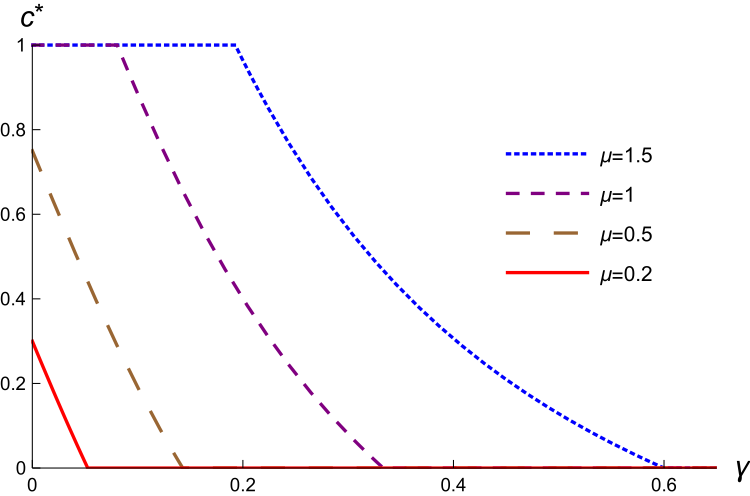
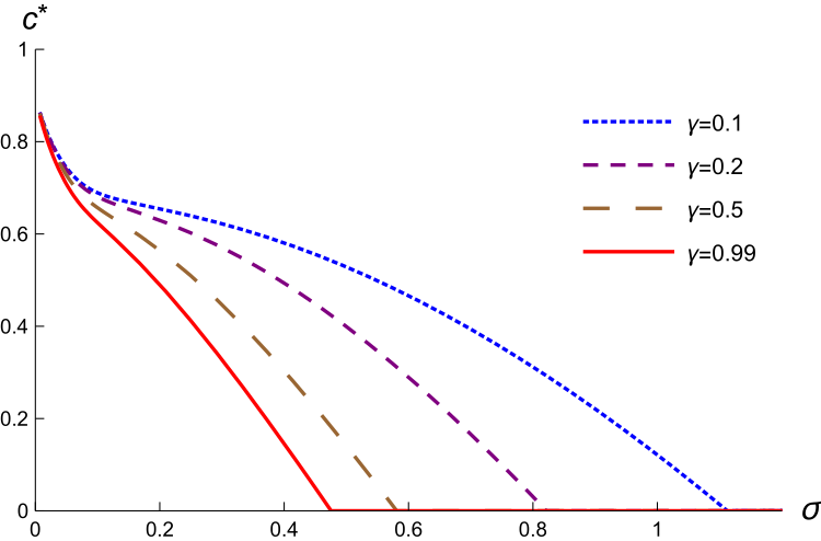
Recall from Corollary 3 that, when combined with boundary conditions, there will be a unique solution for any strictly logconcave type density; moreover, the corresponding interval is then an (unrestricted) optimal mechanism. Given uniqueness, the implicit function theorem can be used to affirm the general comparative statics of Proposition 4; moreover, the first-order condition can also be used to compute numerically the optimal interval threshold for standard distributions. Figure 2 illustrates for Normal distributions. The left panel verifies comparative statics already discussed; note that a higher mean $\mu$ is a likelihood ratio right-shift and hence more alignment. The right panel shows comparative statics in the variance of the distribution. We see that there is less discretion when the variance is lower, with the optimal threshold converging, as $\sigma \to 0$, to Proposer’s optimal offer, $0.9$, to type $\mu =0.45$. $\diamond$

(a) $\sigma =1$.

(b) $\mu =0.45$.

Figure 2: Optimal interval thresholds for Normal distributions (mean $\mu$, variance ${\sigma }^2$) and linear-quadratic Proposer utility, $u(a)=-(1-\gamma )|1-a|-\gamma {(1-a)}^2$.

While we do not have general comparative statics results in the variability of the type distribution, it can be shown that for any strictly unimodal distribution with mode $\mathrm{Mo}\ge 0$, an optimal interval delegation set has more compromise than if Proposer knew Vetoer’s type to be $\mathrm{Mo}$. That is, if $c^{\ast }$ is an optimal interval threshold, then $c^{\ast }\le \min \{2\mathrm{M}\mathrm{o},1\}$; the inequality is strict if $\mathrm{Mo}\in (0,1/2)$. Adding this kind of uncertainty to the complete-information model of Romer and Rosenthal (1978) thus increases the extent of Proposer’s compromise.

Comparative statics with respect to changes in the status quo are ambiguous. In particular, one may conjecture that increasing the status quo from $0$ towards $1$ would reduce the optimal amount of discretion or extent of compromise (i.e., increase $C^{\ast }$, as in Proposition 4 (ii)). This is not assured, however, even in the simplest case of linear loss utility and a strictly logconcave density. To see that, observe using the subgradient condition discussed after Proposition 2 that no compromise can be (uniquely) optimal given our status quo of $0$ for suitable logconcave distributions with mode in $(0,1)$. But if the status quo is raised to some $s$ in between the mode and $1$, then full delegation under the new status quo (i.e., $[s,1]$) becomes optimal. Discretion has increased.

4.2 Comparisons

This subsection compares the outcome of optimal delegation with two game forms considered in earlier work.

A natural starting point is the incomplete-information version of the Romer and Rosenthal (1978) model. Proposer makes a take-it-or-leave it proposal $a\in ℝ$, which Vetoer can accept or veto. This can be viewed as restricting Proposer to singleton delegation sets. Clearly, Proposer is strictly worse off in this institution unless no compromise is the optimal mechanism. We assume throughout this subsection that no compromise is not an optimal interval delegation set; as noted in Subsection 3.2 it is sufficient that Proposer’s utility $u(a)$ is differentiable at his ideal point $a=1$ (hence $u^{\prime }(1)=0$). We will see below that not only does Proposer strictly benefit from optimal delegation, but so does Vetoer under some conditions, even when full delegation is not optimal for Proposer.

Matthews (1989) studies cheap talk before veto bargaining: prior to Proposer making a singleton proposal, Vetoer can send a costless and nonbinding message. As usual in cheap-talk games there is an uninformative and hence noninfluential equilibrium, in which Proposer makes the same proposal, $a_U>0$, as he would absent the possibility of cheap talk. Matthews provides conditions under which there is also an equilibrium with informative and influential cheap talk; it is sufficient given the support of our type density that $u^{\prime }(1)=0$ (or that even the weaker condition in fn. 25 holds). A set of low Vetoer types pool on a “veto threat” message, while the complementary set of high types pool on an “acquiescing” message. In response to the latter message, Proposer offers $a=1$; in response to the veto threat Proposer offers some $a_I\in (0,1)$. The former proposal is accepted by all types that acquiesced, while the latter is accepted by only a subset of types that made the veto threat; types below some strictly positive threshold exercise the veto. An influential cheap-talk equilibrium is outcome equivalent to the delegation set $\{a_I,1\}$ in our framework.

There can be multiple cheap-talk equilibria with distinct outcomes, both among influential equilibria and among noninfluential equilibria (i.e., distinct $a_I$ and $a_U$ respectively). Matthews shows that in any two equilibria of the respective kinds; moreover, he provides conditions under which $a_I$ is unique, i.e., all influential cheap-talk equilibria have the same outcome (Matthews, 1989, Remark 3). As elaborated in the proof of our Proposition 5, multiplicity is ruled out when the following function has a unique zero:

$$2u^{\prime }(a)\left[F((1+a)/2)-F(a/2)\right]-f(a/2)\left[u(a)-u(0)\right].$$ (3)

By way of comparison, we recall that a zero of a similar function given in (2) is the first-order condition for optimality of an interval delegation set’s threshold.

Proposition 5.

Assume no compromise is not an optimal delegation set, and that either (2) or (3) is strictly downcrossing on $(0,1)$. Any optimal interval delegation set $[c^{\ast },1]$ has for any influential and noninfluential cheap-talk equilibrium $a_I$ and $a_U$, respectively. Hence, if $[c^{\ast },1]$ is an optimal delegation set, then it strongly Pareto dominates any cheap-talk outcome, influential or not.

By strong Pareto dominance, we mean that Proposer is ex-ante better off, while Vetoer is better off no matter his type; moreover, a set of Vetoer types that have strictly positive probability are strictly better off. Proposition 5’s conclusions hold trivially when full delegation is the optimal delegation set ($c^{\ast }=0$), even without its hypotheses. But under its hypotheses, the conclusions also apply to other optimal intervals. The function (2) is strictly downcrossing on $(0,1)$ under Condition LQ and either strict logconcavity of the type density or strict concavity of Proposer’s utility. Indeed, this underlies the uniqueness claim in Corollary 3; see Lemma B.1. Moreover, Corollary 3 also assures that interval delegation is then optimal.

Here is the intuition behind Proposition 5. Consider Proposer’s tradeoff when marginally lowering his proposal $a_I\in (0,1)$ in an influential cheap-talk equilibrium. The benefit is that some types just below $a_I/2$ will accept rather than veto; the cost is that the action induced from all types in the interval $(a_I/2,(1+a_I)/2)$ is lower. When Proposer instead delegates the interval $[a_I,1]$, the benefit from lowering $a_I$ is unchanged while the cost is reduced, because types above $a_I$ are now unaffected by the change. Proposer is thus more willing to compromise when choosing among interval delegation sets rather than under cheap talk. Consequently, all Vetoer types benefit—at least weakly, and some strictly—from optimal interval delegation as compared to cheap talk. While Proposer could be harmed by a restriction to interval delegation, there is strong Pareto dominance when intervals constitute optimal delegation.

We note that if interval delegation is not optimal, then some Vetoer types may be worse off under optimal delegation than under cheap talk. For example, it is possible that the optimal delegation set takes the form $\{a^{\ast },1\}$ with $a^{\ast }\in (0,1)$. In this case one can show that necessarily in any influential cheap-talk equilibrium; intuitively, while $a_I$ is sequentially rational, committing to a lower proposal helps ex ante by inducing action $1$ rather than $a_I$ from some types. Consequently, while Proposer strictly benefits from optimal delegation, some Vetoer types would strictly prefer either cheap-talk outcome.

5 Applications

We now discuss some implications and interpretations of our analysis in the context of three applications.

Menus of products.

Our framework can be applied to questions of which products to present customers with, albeit in a stylized manner. For an illustration, suppose a salesperson has at his disposal a set of products indexed by $a\in [0,1]$, with higher $a$ corresponding to higher quality. The price of product $a$ is $k{a}^2$, where $k>0$. This pricing can be interpreted as emerging from a constant markup on a quadratic cost. Consumers vary in how they trade off quality and price; specifically, a consumer of type $v\ge 0$ has gross valuation $va$, and hence net-of-price payoff $va-k{a}^2$. If a consumer does not purchase, his payoff is $0$; a consumer cannot purchase a product he is not shown (perhaps because of ignorance, or because the salesperson can claim it is unavailable). Observe that we can normalize $k=1/2$, as this simply rescales the consumer type $v$. The salesperson receives a higher commission on better products, reflected by his strictly increasing and concave utility $u(a)$. Given any belief density the salesperson holds about a particular consumer’s valuation the salesperson’s problem of which products to show the consumer is precisely that of determining the optimal delegation set in our setting.

Take the case of a linear $u$. Propositions 1–3 imply that if the density of $v$ is logconcave, it is optimal to show the consumer some set of “best products” (i.e., an interval of products $[c,1]$); if the density is strictly decreasing, then all products should be shown; and if the density is strictly increasing, then only the highest-quality product should be shown. Proposition 4(i) implies that if the commission schedule changes to make $u$ more concave, the salesperson shows a larger set of products. Proposition 4(ii) implies that if wealthier consumers (or, if wealth is unobservable, some proxy thereof) have a higher distribution of $v$ in the likelihood ratio sense, then wealthier consumers are shown a smaller set of products.

What if a consumer can choose the information to disclose about her type? Specifically, suppose, as is standard in voluntary disclosure models, that any type $v$ can send any message (a closed subset of ${ℝ}_{+}$) that contains $v$. The salesperson decides on the product menu after observing the message. No matter the type distribution, there are at least two equilibria: one in which no type discloses any information, and one in which all types fully disclose. Every consumer type prefers the former equilibrium to the latter; some types have a strict preference unless nondisclosure results in only a single product being shown (Proposition 2). In general there can be other equilibria, some of which may dominate the nondisclosure equilibrium in terms of ex-ante consumer welfare. However, when the salesperson offers all products under the prior (Proposition 1), the nondisclosure equilibrium is consumer optimal—not only ex ante, but for every consumer type.

Lesser-included offenses.

The legal doctrine of lesser-included offenses in criminal cases is “the concept that a defendant may be found guilty of an uncharged lesser offense, instead of the offenses formally charged …a recognized and well-established feature of the American criminal justice system” (Adlestein, 1995). For instance, “the lesser-included offenses of first degree murder include second degree murder, voluntary manslaughter, involuntary manslaughter, criminally negligent homicide, and aggravated assault” (Orzach and Spurr, 2008). The framework studied in our paper provides a formal lens to understand welfare implications of the doctrine for both prosecutors and defendants.

Our model views $v$ as a jury’s (or judge’s) evaluation of the optimal penalty or true severity of a crime. The defendant is delivered a penalty or sentence corresponding to the most severe charge on which there is a conviction. Verdict $0$ corresponds to a complete acquittal, which is always available to the jury, while $1$ is the maximum penalty or the maximum charge the prosecutor can realistically put forward in a given case. We assume the jury will convict the defendant of the closest charge to $v$ that is available. In a stylized manner, the lesser-included offenses doctrine can be modeled as implying that if a charge $a$ is included, then the jury can choose any verdict in $[0,a]$. Plainly, if a prosecutor has the option to put forward any subset of charges—or equivalently, to have the jury selectively instructed about only specific lesser offenses—then the doctrine (or the jury being instructed of it in full) is just a constraint. It necessarily makes the prosecutor worse off ex ante, at least weakly. It follows that if the defendant’s utility is the additive inverse of the prosecutor’s, then the doctrine can only help the defendant ex ante.

Our analysis clarifies, however, circumstances in which the doctrine does not strictly hurt the prosecutor, or help the defendant, ex ante. Assume the prosecutor’s utility $u$ is increasing in the verdict. Under the doctrine, the prosecutor then brings the maximum charge. So the prosecutor’s ex-ante utility is the same absent the doctrine if and only if full delegation is unconstrained optimal. So long as $u$ is concave, Proposition 1 can be applied; in particular, the doctrine is irrelevant for any prosecutor who is sufficiently risk averse (Corollary 2). On the other hand, from an ex-post perspective, it is precisely when full delegation is not prosecutor optimal that the prosecutor will strictly benefit and the defendant strictly lose, with positive probability, from the doctrine.

The foregoing discussion assumes the prosecutor can bring any set of charges. If the prosecutor were restricted to bringing a single charge, then the welfare implications of the lesser-included offenses doctrine are less clear cut. The issue boils down to whether full delegation is ex-ante preferred by the relevant party to the prosecutor’s optimal single charge. We observe that now the doctrine ex-ante benefits the prosecutor and hurts the defendant when full delegation is unconstrained optimal, whereas the comparison is reversed when no compromise is unconstrained optimal (Proposition 2).

Legislatures and Executives.

Legislatures write bills that can be vetoed by executives. But executives do more than just approve or veto: as emphasized by Epstein and O’Halloran (1996, pp. 378–379), “all laws passed by Congress are implemented by the executive branch in one form or another”, and, since, “Presidents generally appoint administrators with preferences similar to their own” the amount of discretion given is a “key variable in …congressional-executive relations”. One interpretation of our results is that they predict bills granting the executive more discretion when there is greater preference misalignment between the executive and the legislature, in the sense of Proposition 4(ii). This flips the comparative static emphasized in the political science literature (Epstein and O’Halloran, 1996, 1999), which stems from expertise-based delegation models. Of course, in practice one expects both the expertise-based rationale and our veto-based one to coexist to varying degrees.

There are examples of legislatures apparently providing misaligned executives with veto power greater discretion than the legislature would consider optimal. A case in point is the “U.S. Troop Readiness, Veterans’ Care, Katrina Recovery, and Iraq Accountability Appropriations Act” (House Resolution 2206) enacted in May 2007 that provided funding for the United States’ war in Iraq. Congress passed an earlier version, House Resolution 1591, that set a deadline of April 2008 for U.S. troops to withdraw from Iraq. This suggests that, even after accounting for any expertise-based delegation rationale, Congress preferred a relatively tight deadline. But the bill was vetoed by President George W. Bush. Although Democrats controlled both chambers of Congress, they did not have the requisite supermajority to override the veto. To secure the President’s approval, the eventual Act replaced the withdrawal deadline with vague metrics that gave the President more discretion.

We must also stress an alternative perspective on our results: rather than passing bills that grant ex-post discretion, discretion can manifest in the executive effectively selecting which bill (from some subset, none of which grant ex-post discretion) the legislature passes. For example, the President may be consulted by Congress about different versions of legislation. These two forms of discretion are equivalent within our model. An empirical test of our model’s predictions in the political arena would have to overcome this challenge, and that of the coexistence of expertise- and veto-based delegation rationales.

6 Conclusion

We have studied Proposer’s optimal mechanism, absent transfers, in a simple model of veto bargaining. Our main results identify sufficient and necessary conditions for the optimal mechanism to take the form of certain delegation sets, including full delegation, no compromise, and more generally interval delegation. While we have focused on a quadratic loss function for Vetoer, our analytical methodology can be applied to deduce optimality of these delegation sets for a broader class of Vetoer preferences. Specifically, the methods can be readily applied to Vetoer utility functions of the form $va+b(a)$, for any differentiable and strictly concave function $b$. The conditions in Propositions 1–3 would be more complicated, however. Our methodology could also be used to deduce optimality of other kinds of delegation sets, for example Proposer offering his ideal point and one additional compromise option.

In some applications it is plausible that Vetoer can choose among multiple default options. For instance, there may be two internal candidates available to an organization for an open position even if it rejects those put forward by a search committee. Formally, suppose Vetoer has available a finite set of actions to choose among if she exercises her veto. Proposer’s optimal delegation set can be obtained by simply solving a series of separate problems analogous to ours, and then “stitching” the solutions together. Let us illustrate assuming Vetoer has only two options upon a veto, which we denote $0$ and $a^{\ast }>0$. If $a^{\ast }>1$, then Proposer solves the problem we have studied—with a single veto option at $0$—to determine a delegation set $A\subseteq [0,1]$; separately, she solves an analogous problem in which the single veto option is $a^{\ast }$ to determine a delegation set $A^{\prime }\subseteq [1,a^{\ast }]$. The overall optimal delegation set is simply $A\cup A^{\prime }$. If, on the other hand, , then Proposer determines an optimal $A\subseteq [0,a^{\ast }]$ with veto option $0$ and her ideal point viewed as $a^{\ast }$, and an optimal $A^{\prime }\subseteq [a^{\ast },1]$ with the veto option viewed as $a^{\ast }$ and her true ideal point $1$; the overall optimal delegation set is again $A\cup A^{\prime }$. As an example, assume Proposer has linear loss utility and the type distribution is unimodal with mode less than $1$. Following Remark 2, our model’s solution is interval delegation with a threshold at some $c^{\ast }\in [0,1]$. So long as the additional veto option is $a^{\ast }\ge c^{\ast }$, it follows that the solution is unchanged: if $a^{\ast }\in [c^{\ast },1]$, then $a^{\ast }$ was already part of the optimal delegation set; if $a^{\ast }>1$, then the decreasing density to the right of $1$ means, by Proposition 2, that no compromise is optimal on $[1,a^{\ast }]$.

A key assumption underlying our analysis is that of Proposer commitment. In some contexts Proposer may be unable to preclude reapproaching Vetoer with another proposal (or menu of proposals) following a veto. When the optimal mechanism in our setting is full delegation, we believe that such lack of commitment is not problematic. By offering the full-delegation menu to begin with, bargaining will effectively conclude at the first opportunity.

When full delegation is not optimal, however, matters are considerably more nuanced. Sequential veto bargaining without commitment has received only limited theoretical attention, largely in finite-horizon models with particular type distributions (e.g., Cameron, 2000). In ongoing research, we are studying an infinite-horizon model. Our preliminary results suggest that, owing to single-peaked preferences, non-Coasian dynamics can emerge that allow Proposer to obtain her commitment solution when players are patient.

Appendices

Appendix A Proofs of Propositions 1, 2, and 3

In Appendix A we assume the support of the type distribution $F$ is $[0,1]$. This is without loss (even among stochastic mechanisms) because it is always optimal for Proposer to choose action $1$ for types above $1$ and, given the outside option, to choose action $0$ for types below $0$.

A.1 Sufficient Conditions

For convenience, we recall Proposer’s problem (P):

$\underset{m\in 𝒮}{\max }{\displaystyle {\int }_0^1}{𝔼}_{m(v)}[u(a)]dF(v)$ (P)

$\text{s.t. }{𝔼}_{m(v)}\left[av-a^2/2\right]-{\displaystyle {\int }_0^v}{𝔼}_{m(x)}[a]dx=0\forall v\in [0,1].$ (IC-env)

We also recall the relaxed problem (R):

$\underset{\alpha \in 𝒜}{\max }{\displaystyle {\int }_0^1}\left(u(\alpha (v))-\kappa \left[v\alpha (v)-{\displaystyle \frac{\alpha {(v)}^2}{2}}-{\displaystyle {\int }_0^v}\alpha (x)dx\right]\right)dF(v)$ (R)

$\text{s.t. }v\alpha (v)-{\displaystyle \frac{\alpha {(v)}^2}{2}}-{\displaystyle {\int }_0^v}\alpha (x)dx\ge 0\forall v\in [0,1].$

Problem (P) concerns stochastic mechanisms while problem (R) concerns deterministic ones. In general, there need be no deterministic mechanism that solves problem (P). In particular, the solution to problem (R) need not be incentive compatible (as problem (R) only has a relaxed incentive constraint) and hence need not be feasible in problem (P). The example in Appendix E illustrates. However, the following result holds:

Lemma A.1.

Suppose ${\alpha }^{\ast }\in 𝒜$ solves problem (R) and is incentive compatible. Then ${\alpha }^{\ast }$ also solves (P).

• To obtain a contradiction, suppose ${\alpha }^{\ast }$ does not solve (P). Since ${\alpha }^{\ast }$ is, by assumption, feasible for (P), there is $m\in 𝒮$ that is feasible for (P) and achieves a strictly higher objective value in (P) than ${\alpha }^{\ast }$. Define $\overline{\alpha }\in 𝒜$ by setting $\overline{\alpha }(v):={𝔼}_{m(v)}[a]$ for each $v$. It holds that ${\int }_0^v{𝔼}_{m(x)}[a]dx={\int }_0^v\overline{\alpha }(x)ds$, while for any $v$ Jensen’s inequality implies ${𝔼}_{m(v)}\left[av-a^2/2\right]\le v\overline{\alpha }(v)-\overline{\alpha }{(v)}^2/2$. Hence, feasibility of $m$ in (P) implies feasibility of $\overline{\alpha }$ in (R). Moreover,

  ${\displaystyle {\int }_0^1}\left(u(\overline{\alpha }(v))-\kappa \left[v\overline{\alpha }(v)-{\displaystyle \frac{\overline{\alpha }{(v)}^2}{2}}-{\displaystyle {\int }_0^v}\overline{\alpha }(x)dx\right]\right)dF(v)$

  $\ge$ ${\displaystyle {\int }_0^1}\left({𝔼}_{m(v)}\left[u(a)-\kappa \left(va-{\displaystyle \frac{a^2}{2}}\right)\right]+\kappa {\displaystyle {\int }_0^v}{𝔼}_{m(x)}[a]dx\right)dF(v)$

  $=$ ${\displaystyle {\int }_0^1}{𝔼}_{m(v)}[u(a)]dF(v)$

  $>$ ${\displaystyle {\int }_0^1}u({\alpha }^{\ast }(v))dF(v)$

  $=$ ${\displaystyle {\int }_0^1}\left(u({\alpha }^{\ast }(v))-\kappa \left[v{\alpha }^{\ast }(v)-{\displaystyle \frac{{\alpha }^{\ast }{(v)}^2}{2}}-{\displaystyle {\int }_0^v}{\alpha }^{\ast }(x)dx\right]\right)dF(v),$

  where the first inequality holds because the first line is a concave functional (by the definition of $\kappa \equiv {inf}_{a\in [0,1)}-u^{\prime \prime }(a)$), the first equality holds because $m$ is feasible in (P), the second inequality holds because of our assumption that $m$ achieves a strictly higher value than ${\alpha }^{\ast }$, and the final equality holds because ${\alpha }^{\ast }$ being IC implies it is feasible in (P). Therefore, ${\alpha }^{\ast }$ is not optimal in (R), a contradiction. ∎

To show that a given delegation set solves the relaxed problem, we define a Lagrangian functional and use the fact, stated as Lemma A.2 below, that it is enough to find a Lagrangian multiplier such that the action rule induced by the delegation set maximizes the Lagrangian with that multiplier. Given $\alpha \in 𝒜$ and an increasing and right-continuous function $\mathrm{\Lambda }(v)$, let the Lagrangian be given by

$ℒ(\alpha ,\mathrm{\Lambda })$ $:={\displaystyle {\int }_0^1}\left(u(\alpha (v))f(v)-\kappa f(v)\left[v\alpha (v)-{\displaystyle \frac{\alpha {(v)}^2}{2}}-{\displaystyle {\int }_0^v}\alpha (x)dx\right]\right)dv$

$+{\displaystyle {\int }_0^1}\left(v\alpha (v)-{\displaystyle \frac{\alpha {(v)}^2}{2}}-{\displaystyle {\int }_0^v}\alpha (x)dx\right)d\mathrm{\Lambda }(v)$

$={\displaystyle {\int }_0^1}\left(u(\alpha (v))f(v)-\alpha (v)[\kappa F(v)-\mathrm{\Lambda }(v)]-\kappa f(v)\left[v\alpha (v)-{\displaystyle \frac{\alpha {(v)}^2}{2}}\right]\right)dv$

$+{\displaystyle {\int }_0^1}\left(v\alpha (v)-{\displaystyle \frac{\alpha {(v)}^2}{2}}\right)d\mathrm{\Lambda }(v)+{\displaystyle {\int }_0^1}\alpha (v)dv[\kappa F(1)-\mathrm{\Lambda }(1)],$ (A.1)

where the second equality follows from integration by parts.

Lemma A.2.

Let ${\alpha }^{\ast }$ be induced by a delegation set. Suppose there is an increasing and right-continuous function $\mathrm{\Lambda }$ such that $ℒ({\alpha }^{\ast },\mathrm{\Lambda })\ge ℒ(\alpha ,\mathrm{\Lambda })$ for all $\alpha \in 𝒜$. Then ${\alpha }^{\ast }$ solves problem (R).

Here is the idea. Since ${\alpha }^{\ast }$ is incentive compatible (as it is induced by a delegation set), it is feasible for the relaxed problem (R) and satisfies all inequality constraints as equalities. This implies that complementary slackness is satisfied for any Lagrange multiplier $\mathrm{\Lambda }$. It follows that ${\alpha }^{\ast }$ solves problem (R) if it maximizes the Lagrangian functional.

• Let $Obj(\alpha )$ denote the value of the objective function in problem (R) with mechanism $\alpha$. Since ${\alpha }^{\ast }$ is incentive compatible,

  $$v{\alpha }^{\ast }(v)-\frac{{\alpha }^{\ast }{(v)}^2}{2}-{\int }_0^v{\alpha }^{\ast }(x)dx=0,$$

  and therefore $Obj({\alpha }^{\ast })=ℒ({\alpha }^{\ast },\mathrm{\Lambda })$. For any $\alpha \in 𝒜$ that is feasible for (R),

  $$v\alpha (v)-\frac{\alpha {(v)}^2}{2}-{\int }_0^v\alpha (x)dx\ge 0;$$

  since $\mathrm{\Lambda }$ is non-decreasing, this implies $ℒ(\alpha ,\mathrm{\Lambda })\ge Obj(\alpha )$. We conclude

  $$Obj({\alpha }^{\ast })=ℒ({\alpha }^{\ast },\mathrm{\Lambda })\ge ℒ(\alpha ,\mathrm{\Lambda })\ge Obj(\alpha ).\mathit{∎}$$

To apply Lemma A.2, we will use a first-order approach, i.e., for the action rule $\alpha$ induced by the desired delegation set, we construct a multiplier and verify that given this multiplier the Lagrangian’s Gateaux differential at $\alpha$ is negative in any feasible direction. This approach is valid so long as the constructed multiplier makes the Lagrangian a concave functional (Luenberger, 1969, Lemma 1 and its proof on p. 227). The following observation will allow us to establish the Lagrangian’s concavity.

Lemma A.3.

Suppose $K:[0,1]\to ℝ$ is right-continuous and increasing and $h:{ℝ}^2\to ℝ$ is bounded, measurable, and for each value of its second argument concave in its first argument. Then $S:L^{\mathrm{\infty }}\to ℝ$ defined by $S(\alpha ):={\int }_0^{1}h(\alpha (v),v)dK(v)$ is concave.

• Fix ${\alpha }_1,{\alpha }_2\in L^{\mathrm{\infty }}$, $c\in (0,1)$ and let ${\alpha }_c=c{\alpha }_1+(1-c){\alpha }_2$. Then

  $S({\alpha }_c)-cS({\alpha }_1)-(1-c)S({\alpha }_2)={\displaystyle {\int }_0^1}\left(h({\alpha }_c(v),v)-ch({\alpha }_1(v),v)-(1-c)h({\alpha }_2(v),v)\right)dK(v)\ge 0$

  because concavity of $h$ implies that the integrand is positive for each $v$ and because $K$ is increasing. ∎

Note that for each $v$, $u(\alpha (v))f(v)+\kappa f(v)\frac{\alpha {(v)}^2}{2}$ is concave in $\alpha (v)$ since its second derivative is given by $f(v)[u^{\prime \prime }(\alpha (v))+\kappa ]$, which is negative by definition of $\kappa$. This implies that, for each $v$, each integrand in (A.1) is a concave function of $\alpha (v)$. Hence, if $\mathrm{\Lambda }$ is right-continuous and increasing, Lemma A.3 implies that the Lagrangian $ℒ(\alpha ,\mathrm{\Lambda })$ is concave in $\alpha$.

We will construct right-continuous and increasing multipliers $\mathrm{\Lambda }$ that, for ease of calculations, also satisfy $\mathrm{\Lambda }(1)=\kappa F(1)$. With this equality, (A.1) simplifies to

$ℒ(\alpha ,\mathrm{\Lambda })$ $={\displaystyle {\int }_0^1}\left(u(\alpha (v))f(v)-\alpha (v)[\kappa F(v)-\mathrm{\Lambda }(v)]-\kappa f(v)\left[v\alpha (v)-{\displaystyle \frac{\alpha {(v)}^2}{2}}\right]\right)dv$

$+{\displaystyle {\int }_0^1}\left(v\alpha (v)-{\displaystyle \frac{\alpha {(v)}^2}{2}}\right)d\mathrm{\Lambda }(v),$

and the Gateaux differential in the direction of mechanism $\overline{\alpha }$ is

$\partial ℒ(\alpha ,\overline{\alpha },\mathrm{\Lambda })$ $={\displaystyle {\int }_0^1}\left(\left[u^{\prime }\left(\alpha \left(v\right)\right)f\left(v\right)-\kappa F\left(v\right)+\mathrm{\Lambda }\left(v\right)\right]\overline{\alpha }\left(v\right)\right)dv+{\displaystyle {\int }_0^1}\left(\left[v-\alpha \left(v\right)\right]\overline{\alpha }\left(v\right)\right)\mathrm{d}\left[\mathrm{\Lambda }\left(v\right)-\kappa F\left(v\right)\right]$ (A.2)

$={\displaystyle {\int }_0^1}\left({\displaystyle {\int }_v^1}{u}^{\prime }\left(\alpha \left(x\right)\right)f\left(x\right)-\kappa F\left(x\right)+\mathrm{\Lambda }\left(x\right)\mathrm{d}x\right)d\overline{\alpha }\left(v\right)+{\displaystyle {\int }_0^1}\left({\displaystyle {\int }_v^1}\left[x-\alpha \left(x\right)\right]\mathrm{d}\left[\mathrm{\Lambda }\left(x\right)-\kappa F\left(x\right)\right]\right)d\overline{\alpha }\left(v\right),$ (A.3)

where the second equality obtains using integration by parts.

Putting everything together, the sufficiency direction of each of Propositions 1, 2, and 3 can now be proven by constructing a right-continuous and increasing multiplier $\mathrm{\Lambda }$ such that $\mathrm{\Lambda }(1)=\kappa F(1)$, and showing that for $\alpha$ induced by the relevant delegation set and for all $\overline{\alpha }\in 𝒜$, the Gateaux differential in the direction of $\overline{\alpha }-\alpha$, computed using (A.2) or (A.3), is negative.

• The action rule induced by full delegation is $\alpha (v)=v$. We claim that $\alpha$ maximizes the Lagrangian for the multiplier $\mathrm{\Lambda }(v):=\kappa F(v)-u^{\prime }(v)f(v)$ for and $\mathrm{\Lambda }(1):=\kappa F(1)$. Note that the multiplier is increasing since $\kappa F(v)-u^{\prime }(v)f(v)$ is increasing by assumption and $u^{\prime }(v)\ge 0$. The Lagrangian is therefore maximized at $\alpha$ if $\partial ℒ(\alpha ,\overline{\alpha }-\alpha ,\mathrm{\Lambda })\le 0$ for all $\overline{\alpha }\in 𝒜$. Note that the integrand of the first integral in (A.2) is 0 for almost every $v$ by choice of $\mathrm{\Lambda }$ and the second integral is 0 since $\alpha (v)=v$. ∎

We next consider the optimality of no compromise.

• The action rule induced by no compromise satisfies $\alpha (v)=0$ for $v\in [0,\frac{1}{2})$ and $\alpha (v)=1$ for $v\in [\frac{1}{2},1]$. Now suppose for all $s\in [0,1/2)$ and $t\in (1/2,1]$ we have

  $$(u^{\prime }(1)+\kappa (1-t))\frac{F(t)-F(1/2)}{t-1/2}\ge (u^{\prime }(0)-\kappa s)\frac{F(1/2)-F(s)}{1/2-s}.$$

  and let $\psi :={inf}_{t\in (1/2,1]}(u^{\prime }(1)+\kappa (1-t))\frac{F(t)-F(1/2)}{t-1/2}$. Define $\mathrm{\Lambda }(v):=\kappa F(1/2)-\psi$ for $v\in [0,1)$ and $\mathrm{\Lambda }(1):=\kappa F(1)$.

  Let $s\in (1/2,1]$. Integrating by parts, ${\int }_s^{1/2}vdF(v)=1/2F(1/2)-sF(s)-{\int }_s^{1/2}F(v)dv$. Since $\mathrm{\Lambda }(v)$ is constant on $[0,1)$, the definition of $\psi$ implies that, for any $s\in [0,1/2)$,

  ${\displaystyle {\int }_s^{1/2}}{u}^{\prime }(\alpha (v))f(v)-\kappa F(v)+\mathrm{\Lambda }(v)\mathrm{d}v+{\displaystyle {\int }_s^{1/2}}v\mathrm{d}[\mathrm{\Lambda }(v)-\kappa F(v)]$

  $=$ $u^{\prime }(0)[F(1/2)-F(s)]-1/2[\mathrm{\Lambda }(1/2)-\kappa F(1/2)]-s[\mathrm{\Lambda }(s)-\kappa F(s)]$

  $=$ $[u^{\prime }(0)+\kappa s][F(1/2)-F(s)]-(1/2-s)\psi \le 0.$ (A.4)

  Similarly, for any $t\in (1/2,1]$,

  ${\displaystyle {\int }_{1/2}^t}{u}^{\prime }(\alpha (v))f(v)-\kappa F(v)+\mathrm{\Lambda }(v)\mathrm{d}v+{\displaystyle {\int }_{1/2}^t}[v-\alpha (v)]\mathrm{d}[\mathrm{\Lambda }(v)-\kappa F(v)]$

  $=$ $u^{\prime }(1)[F(t)-F(1/2)]+(t-1)[\mathrm{\Lambda }(t)-\kappa F(t)]+1/2[\mathrm{\Lambda }(1/2)-\kappa F(1/2)]$

  $=$ $[u^{\prime }(1)+\kappa (1-t)][F(t)-F(1/2)]-(t-1/2)\psi \ge 0.$ (A.5)

  Fix arbitrary $\overline{\alpha }\in 𝒜$ that satisfies $\overline{\alpha }(1)=1$. It follows from (A.3) and the definition of $\alpha$ that

  $\partial ℒ(\alpha ,\overline{\alpha }-\alpha ,\mathrm{\Lambda })$

  $=$ ${\displaystyle {\int }_0^1}\left[{\displaystyle {\int }_v^1}(u^{\prime }(\alpha (x))f(x)-\kappa F(x)+\mathrm{\Lambda }(x))dx+{\displaystyle {\int }_v^1}([x-\alpha (x)]\mathrm{d}[\mathrm{\Lambda }(x)-\kappa F(x)])\right]\mathrm{d}[\overline{\alpha }(v)-\alpha (v)]$

  $=$ ${\displaystyle {\int }_0^1}\left[{\displaystyle {\int }_v^{1/2}}(u^{\prime }(\alpha (x))f(x)-\kappa F(x)+\mathrm{\Lambda }(x))dx+{\displaystyle {\int }_v^{1/2}}([x-\alpha (x)]\mathrm{d}[\mathrm{\Lambda }(x)-\kappa F(x)])\right]d\overline{\alpha }(v).$

  Since $\overline{\alpha }$ is increasing, (A.4) and (A.5) imply that $\partial ℒ(\alpha ,\overline{\alpha }-\alpha ,\mathrm{\Lambda })\le 0$. Since the optimal action rule chooses action 1 for type 1, and we have shown that changes in the direction of any allocation rule that assigns action 1 to type 1 is not an improvement over $\alpha$, we conclude that $\alpha$ is optimal. ∎

Lastly, we consider optimality of interval delegation.

• The action rule induced by interval delegation is $\alpha (v)=0$ for , $\alpha (v)=c^{\ast }$ for $c^{\ast }/2\le v\le c^{\ast }$ and $\alpha (v)=v$ for $v>c^{\ast }$. We propose the following multiplier:

  $\mathrm{\Lambda }$ is constant on $[0,c^{\ast })$ and it follows from Proposition 3’s condition (i) that $\mathrm{\Lambda }$ is increasing on $(c^{\ast },1]$. To see that $\mathrm{\Lambda }$ is increasing at $c^{\ast }$, note that condition (ii) holds as an equality for $t=c^{\ast }$ and hence the derivative of the LHS of condition (ii) with respect to $t$ must be negative at $t=c^{\ast }$, which yields

  $$-\kappa \frac{F(c^{\ast })-F(c^{\ast }/2)}{c^{\ast }/2}+u^{\prime }(c^{\ast })\frac{f(c^{\ast })c^{\ast }/2-(F(c^{\ast })-F(c^{\ast }/2))}{{(c^{\ast }/2)}^2}\le 0.$$

  Hence, $\mathrm{\Lambda }$ is increasing at $c^{\ast }$. It is thus sufficient to show $\partial ℒ(\alpha ,\overline{\alpha }-\alpha ,\mathrm{\Lambda })\le 0$ for all $\overline{\alpha }\in 𝒜$.

  Note that, for $v\in [c^{\ast },1]$, $v-\alpha (v)=0$ and the definition of $\mathrm{\Lambda }$ implies that for $v\in [c^{\ast },1)$,

  $u^{\prime }(\alpha (v))f(v)-\kappa F(v)+\mathrm{\Lambda }(v)=0.$

  Therefore,

  $\partial ℒ(\alpha ,\overline{\alpha }-\alpha ,\mathrm{\Lambda })$ $={\displaystyle {\int }_0^{c^{\ast }}}\left({\displaystyle {\int }_v^{c^{\ast }}}{u}^{\prime }(\alpha (x))f(x)-\kappa F(x)+\mathrm{\Lambda }(x)\mathrm{d}s\right)\mathrm{d}[\overline{\alpha }(v)-\alpha (v)]$

  $+{\displaystyle {\int }_0^{c^{\ast }}}\left({\displaystyle {\int }_v^{c^{\ast }}}[x-\alpha (x)]\mathrm{d}[\mathrm{\Lambda }(x)-\kappa F(x)]\right)\mathrm{d}[\overline{\alpha }(v)-\alpha (v)]$

  Since $\alpha$ is constant on $[0,c^{\ast }/2)$ and $[c^{\ast }/2,c^{\ast }]$, $\overline{\alpha }-\alpha$ is increasing on $[0,c^{\ast }/2)$ and $[c^{\ast }/2,c^{\ast }]$. Hence, the following conditions are sufficient for $\alpha$ to maximize the Lagrangian:

  $${\int }_t^{c^{\ast }}\left(u^{\prime }(c^{\ast })f(v)-[\kappa F(v)-\mathrm{\Lambda }(v)]\right)𝑑v+{\int }_t^{c^{\ast }}(v-c^{\ast })d[\mathrm{\Lambda }(v)-\kappa F(v)]\le 0$$

  for $t\in [c^{\ast }/2,c^{\ast }]$, with equality at $t=c^{\ast }/2$, and

  $${\int }_s^{c^{\ast }/2}\left(u^{\prime }(0)f(v)-[\kappa F(v)-\mathrm{\Lambda }(v)]\right)dv+{\int }_s^{c^{\ast }/2}v\mathrm{d}[\mathrm{\Lambda }(v)-\kappa F(v)]\le 0$$

  for $s\in [0,c^{\ast }/2)$.

  Note that ${\int }_t^{c^{\ast }}\left(F(v)+(v-c^{\ast })f(v)\right)dv=(c^{\ast }-t)F(t)$ and $\mathrm{\Lambda }$ is constant on $[0,c^{\ast })$. Hence, using the definition of $\mathrm{\Lambda }$, we get that for $t\in [c^{\ast }/2,c^{\ast }]$,

  ${\displaystyle {\int }_t^{c^{\ast }}}\left(u^{\prime }(c^{\ast })f(v)-[\kappa F(v)-\mathrm{\Lambda }(v)]\right)dx+{\displaystyle {\int }_t^{c^{\ast }}}(v-c^{\ast })\mathrm{d}[\mathrm{\Lambda }(v)-\kappa F(v)]$

  $=$ ${\displaystyle {\int }_t^{c^{\ast }}}\left(u^{\prime }(c^{\ast })f(v)-\left[\kappa F(v)-\kappa F(c^{\ast }/2)+{\displaystyle \frac{1}{c^{\ast }-c^{\ast }/2}}{\displaystyle {\int }_{c^{\ast }/2}^{c^{\ast }}}{u}^{\prime }(c^{\ast })dF(x)\right]\right)dv-\kappa {\displaystyle {\int }_t^{c^{\ast }}}(v-c^{\ast })dF(v)$

  $=$ $u^{\prime }(c^{\ast })[F(c^{\ast })-F(t)]-u^{\prime }(c^{\ast })[F(c^{\ast })-F(c^{\ast }/2)]{\displaystyle \frac{c^{\ast }-t}{c^{\ast }-c^{\ast }/2}}+\kappa (c^{\ast }-t)[F(c^{\ast }/2)-F(t)]$

  $=$ $-[u^{\prime }(c^{\ast })+\kappa (c^{\ast }-t)][F(t)-F(c^{\ast }/2)]+(t-c^{\ast }/2)u^{\prime }(c^{\ast }){\displaystyle \frac{F(c^{\ast })-F(c^{\ast }/2)}{c^{\ast }-c^{\ast }/2}}$

  $\le$ $0,$

  where the inequality is by Proposition 3’s condition (ii), and holds with equality for $t=c^{\ast }/2$.

  Analogously, note that ${\int }_s^{c^{\ast }/2}F(v)+vf(v)\mathrm{d}v=c^{\ast }/2F(c^{\ast }/2)-sF(s)$ and $\mathrm{\Lambda }$ is constant on $[0,c^{\ast }/2]$. Hence, for $s\in [0,c^{\ast }/2]$,

  ${\displaystyle {\int }_s^{c^{\ast }/2}}\left(u^{\prime }(0)f(v)-[\kappa F(v)-\mathrm{\Lambda }(v)]\right)dv+{\displaystyle {\int }_s^{c^{\ast }/2}}v\mathrm{d}[\mathrm{\Lambda }(v)-\kappa F(v)]$

  $=$ $u^{\prime }(0)[F(c^{\ast }/2)-F(s)]+\mathrm{\Lambda }(s)(c^{\ast }/2-s)-\kappa [c^{\ast }/2F(c^{\ast }/2)-sF(s)]$

  $=$ $[u^{\prime }(0)-\kappa s][F(c^{\ast }/2)-F(s)]-u^{\prime }(c^{\ast }){\displaystyle \frac{F(c^{\ast })-F(c^{\ast }/2)}{c^{\ast }-c^{\ast }/2}}(c^{\ast }/2-s)$

  $\le$ $0,$

  where the inequality is by Proposition 3’s condition (iii). Hence, $\alpha$ is optimal. ∎

A.2 Necessary Conditions

Lemma A.4.

Suppose Condition LQ holds. If ${\alpha }^{\ast }$ is deterministic and solves problem (P) then it also solves problem (R).

• The proof is by contraposition: assuming there exists $\alpha \in 𝒜$ that is feasible for (R) and achieves a strictly higher objective value in (R) than ${\alpha }^{\ast }$, we will construct a solution to (P) that achieves a strictly higher objective value than ${\alpha }^{\ast }$.

Claim 1: There exists $\tilde{\alpha }\in 𝒜$ that is feasible for (R), satisfies $\tilde{\alpha }(v)\le 1$ for all $v$, $v\tilde{\alpha }(v)-\frac{\tilde{\alpha }{(v)}^2}{2}-{\int }_0^v\tilde{\alpha }(s)ds=0$ for all $v$ such that $\tilde{\alpha }(v)=1$, and achieves a weakly higher objective value in problem (R) than $\alpha$.

We can assume $\alpha (v)\le 1$ since $u$ is decreasing above $1$. Now suppose instead that $v\alpha (v)-\frac{\alpha {(v)}^2}{2}-{\int }_0^v\alpha (s)ds>0$ for some $v$ such that $\alpha (v)=1$. Consider an auxiliary setting in which a principal chooses a pair of functions $(\alpha ,t)$ and an agent with type $v$ gets utility $v\alpha (v)-\frac{\alpha {(v)}^2}{2}-t(v)$. Since $\alpha$ is monotonic, it follows from standard arguments that there exist transfers $t:[0,1]\to ℝ$ such that $(\alpha ,t)$ is incentive compatible in the auxiliary setting (e.g., Amador and Bagwell, 2013). For all $v$, these transfers satisfy $t(v)-t(0)=v\alpha (v)-\frac{\alpha {(v)}^2}{2}-{\int }_0^v\alpha (s)ds\ge 0$, where the inequality holds because $\alpha$ is feasible for (R). Define $(\tilde{\alpha },\tilde{t})$ by setting $(\tilde{\alpha }(v),\tilde{t}(v))=(\alpha (v),t(v))$ or $(\tilde{\alpha }(v),\tilde{t}(v))=(1,t(0))$, whichever gives an agent with type $v$ higher expected utility (and choosing the latter if type $v$ is indifferent). Note that $\tilde{t}(0)=t(0)$, which together with $t(v)\ge t(0)$ implies $\tilde{t}(v)-\tilde{t}(0)\ge 0$, with equality for any $v$ such that $\tilde{\alpha }(v)=1$.

Observe that $(\tilde{\alpha },\tilde{t})$ corresponds to an incentive compatible direct mechanism: indeed, if type $v$ strictly prefers $(\tilde{\alpha }(v^{\prime }),\tilde{t}(v^{\prime }))$ to $(\tilde{\alpha }(v),\tilde{t}(v))$ then $v$ also strictly prefers $(\alpha (v^{\prime }),t(v^{\prime }))$ to $(\alpha (v),t(v))$, contradicting the assumption that $(\alpha ,t)$ is incentive compatible. It follows from the standard characterization of incentive compatible mechanisms that $\tilde{\alpha }$ is increasing, and

$$v\tilde{\alpha }(v)-\frac{\tilde{\alpha }{(v)}^2}{2}-{\int }_0^v\tilde{\alpha }(s)ds=\tilde{t}(v)-\tilde{t}(0)\ge 0,$$

with the inequality holding as equality for $v$ such that $\tilde{\alpha }(v)=1$.

Finally, note that $\alpha (v)\le \tilde{\alpha }(v)\le 1$ for all $v$. Also, $\tilde{t}(v)-\tilde{t}(0)\le t(v)-t(0)$, which implies

$$v\tilde{\alpha }(v)-\frac{\tilde{\alpha }{(v)}^2}{2}-{\int }_0^v\tilde{\alpha }(s)ds\le v\alpha (v)-\frac{\alpha {(v)}^2}{2}-{\int }_0^v\alpha (s)ds.$$

It follows that $\tilde{\alpha }$ achieves a weakly higher objective value in problem (R). $\diamond$

Claim 2: Let $\tilde{\alpha }\in 𝒜$ be feasible for (R) and satisfy $\tilde{\alpha }(v)\le 1$ and $v\tilde{\alpha }(v)-\tilde{\alpha }{(v)}^2/2-{\int }_0^v\tilde{\alpha }(s)ds=0$ for all $v$ such that $\tilde{\alpha }(v)=1$. There is a stochastic mechanism $m$ such that, for all $v$, ${Prob}_{m(v)}(a\le 1)=1$, ${𝔼}_{m(v)}[a]=\tilde{\alpha }(v)$, and ${𝔼}_{m(v)}\left[va-\frac{a^2}{2}\right]-{\int }_0^v{𝔼}_{m(s)}[a]ds=0$.

Intuitively, this is because Vetoer’s utility function is quadratic and we can use noise as a substitute for transfers. We provide an explicit construction of the mechanism $m$ below.

For any $v$ such that $\tilde{\alpha }(v)=1$, define $m(v)$ to put mass 1 on action 1. Now fix arbitrary $v$ such that and arbitrary $d\in (-\mathrm{\infty },0]$ and let $t_1(d)=\frac{1-\tilde{\alpha }(v)}{1-d}$. Then $t_1(d)d+(1-t_1(d))1=\tilde{\alpha }(v)$ for all $d$. Moreover, for any $r\in ℝ$ we can choose $d\in (-\mathrm{\infty },0]$ small enough such that

$$-\frac{1-\tilde{\alpha }(v)}{1-d}{d}^2-\left(1-\frac{1-\tilde{\alpha }(v)}{1-d}\right)\le r$$

because the LHS $\to -\mathrm{\infty }$ as $d\to -\mathrm{\infty }$. Hence, by choosing $d$ small enough we get

$$v\tilde{\alpha }(v)-t_1(d)\frac{d^2}{2}-(1-t_1(d))\frac{1}{2}-{\int }_0^v\tilde{\alpha }(s)ds\le 0.$$

Given $v\in [0,1]$ and $t_2\in [0,1]$, we define $m(v)$ to put probability $t_2$ on action $\tilde{\alpha }(v)$, probability $(1-t_2)t_1(d)$ on action $d$, and probability $(1-t_2)(1-t_1(d))$ on action $1$. It follows from the above that $m(v)$ satisfies ${𝔼}_{m(v)}[a]=\tilde{\alpha }(v)$, ${Prob}_{m(v)}(a\le 1)=1$, and we can choose $t_2\in [0,1]$ such that

$${𝔼}_{m(v)}\left[va-\frac{a^2}{2}\right]-{\int }_0^v{𝔼}_{m(s)}[a]ds=0.$$

Defining $m(v)$ in this way for all $v$ such that , the claim follows. $\diamond$

We conclude that $m$ is feasible for (P). Therefore,

${\displaystyle {\int }_0^1}u({\alpha }^{\ast }(v))dF(v)=$ ${\displaystyle {\int }_0^1}\left(u({\alpha }^{\ast }(v))-\kappa \left[v{\alpha }^{\ast }(v)-{\displaystyle \frac{{\alpha }^{\ast }{(v)}^2}{2}}-{\displaystyle {\int }_0^v}{\alpha }^{\ast }(s)ds\right]\right)dF(v)$

${\displaystyle {\int }_0^1}\left(u(\alpha (v))-\kappa \left[v\alpha (v)-{\displaystyle \frac{\alpha {(v)}^2}{2}}-{\displaystyle {\int }_0^v}\alpha (s)ds\right]\right)dF(v)$

$\le$ ${\displaystyle {\int }_0^1}\left(u(\tilde{\alpha }(v))-\kappa \left[v\tilde{\alpha }(v)-{\displaystyle \frac{\tilde{\alpha }{(v)}^2}{2}}-{\displaystyle {\int }_0^v}\tilde{\alpha }(s)ds\right]\right)dF(v)$ (A.6)

where the equality holds because ${\alpha }^{\ast }$ is feasible for (P), the first inequality holds because we assume that $\alpha$ achieves a strictly higher value than ${\alpha }^{\ast }$, and the second inequality holds by Claim 1.

Under Condition LQ, $\kappa \equiv {inf}_{v\in [0,1)}-u^{\prime \prime }(v)=2\gamma$. Hence, for any $a,b\le 1$ and $\lambda \in [0,1]$, some algebra shows that

$$u\left(\lambda a+(1-\lambda )b\right)+\kappa \frac{{\left[\lambda a+(1-\lambda )b\right]}^2}{2}=\lambda \left[u(a)+\kappa \frac{a^2}{2}\right]+(1-\lambda )\left[u(b)+\kappa \frac{b^2}{2}\right].$$

Since ${Prob}_{m(v)}(a\le 1)=1$ and ${𝔼}_{m(v)}[a]=\tilde{\alpha }(v)$ for all $v$, expression (A.6) therefore equals

${\displaystyle {\int }_0^1}\left({𝔼}_{m(v)}\left[u(a)-\kappa \left(va-{\displaystyle \frac{a^2}{2}}\right)\right]+\kappa {\displaystyle {\int }_0^v}{𝔼}_{m(s)}[a]ds\right)dF(v).$

Since $m$ is feasible for (P), this expression equals ${\int }_0^1{𝔼}_{m(v)}[u(a)]dF(v)$. This contradicts the assumption that ${\alpha }^{\ast }$ solves (P), and we conclude that ${\alpha }^{\ast }$ solves (R). ∎

Recall that $Obj(\alpha )$ denotes the value of the objective function in problem (R) with mechanism $\alpha$. The set of feasible solutions for (R) is convex, and optimality of $\alpha$ therefore implies $\partial Obj(\alpha ,\overline{\alpha }-\alpha )\le 0$ for any $\overline{\alpha }\in 𝒜$ that is feasible for (R) (Luenberger, 1969, Theorem 2 on p. 178). Recall the assumption $F(1)=1$. We have:

$Obj(\alpha )$ $={\displaystyle {\int }_0^1}\left(u(\alpha (v))-\kappa \left[v\alpha (v)-{\displaystyle \frac{\alpha {(v)}^2}{2}}-{\displaystyle {\int }_0^v}\alpha (s)ds\right]\right)dF(v),$

$\partial Obj(\alpha ,\overline{\alpha }-\alpha )$ $={\displaystyle {\int }_0^1}\left([u^{\prime }(\alpha (v))-\kappa [v-\alpha (v)]](\overline{\alpha }(v)-\alpha (v))+\kappa {\displaystyle {\int }_0^v}\overline{\alpha }(s)-\alpha (s)\mathrm{d}s\right)dF(v)$

$={\displaystyle {\int }_0^1}\left[u^{\prime }(\alpha (v))-\kappa \left[v-\alpha (v)-{\displaystyle \frac{1-F(v)}{f(v)}}\right]\right](\overline{\alpha }(v)-\alpha (v))dF(v).$ (A.7)

Lemma A.5.

Suppose Condition LQ holds. If a delegation set containing the interval $[a,b]\subseteq [0,1]$ is optimal, then $\kappa F(v)-u^{\prime }(v)f(v)$ is increasing on $[a,b]$.

• Suppose a delegation set containing the interval $[a,b]$ is optimal, and let $\alpha$ denote the corresponding allocation rule. Suppose to the contrary that $\kappa F(v)-u^{\prime }(v)f(v)$ is not increasing on $[a,b]$; since $\kappa F(v)-u^{\prime }(v)f(v)$ is continuously differentiable, there is then an interval $[d,e]\subset [a,b]$ with on which it is strictly decreasing.

  Set

  and observe that $\overline{\alpha }$ is feasible for (R), since it is corresponds to a delegation set obtained by removing $(d,e)$ from the original delegation set. Moreover,

  $\partial Obj(\alpha ,\overline{\alpha }-\alpha )$ $={\displaystyle {\int }_d^e}\left[u^{\prime }(v)f(v)-\kappa F(v)+\kappa \right][\overline{\alpha }(v)-v]dv$

  $>{\displaystyle {\int }_d^e}\left[u^{\prime }\left({\displaystyle \frac{d+e}{2}}\right)f\left({\displaystyle \frac{d+e}{2}}\right)-\kappa F\left({\displaystyle \frac{d+e}{2}}\right)+\kappa \right][\overline{\alpha }(v)-v]dv$

  $=0,$

  where the first equality follows from (A.7) because $\overline{\alpha }(v)=\alpha (v)$ for $v\notin [d,e]$ and $\alpha (v)=v$ for $v\in [d,e]$; the inequality holds because $u^{\prime }(v)f(v)-\kappa F(v)$ is strictly increasing on $[d,e]$ while $\overline{\alpha }(v)-v$ is strictly negative on $(d,\frac{d+e}{2})$ and strictly positive on $(\frac{d+e}{2},e)$; and the final equality holds because ${\int }_d^e[\overline{\alpha }(v)-v]dv=0$. We conclude that $\alpha$ is not optimal. ∎

• Suppose Condition LQ holds. The result follows directly from Lemma A.5. ∎

• Suppose Condition LQ holds and let $\alpha \in 𝒜$ be the action rule induced by the delegation set $\{0,1\}$. Fix $s\in (0,1/2)$ and $t\in (1/2,1)$, $\epsilon \in (0,1)$ and define

  We claim that for any $\epsilon >0$ small enough (so that and ), ${\overline{\alpha }}_{\epsilon }$ is feasible for (R). By definition of ${\overline{\alpha }}_{\epsilon }$, ${\int }_0^v{\overline{\alpha }}_{\epsilon }(s)ds={\int }_0^v\alpha (s)ds$ for all $v\notin (s,t)$. Combining this equality with $\alpha$ being feasible for (R) and ${\overline{\alpha }}_{\epsilon }(v)=\alpha (v)$ for all $v\notin [s,t]$, it follows that

  $v{\overline{\alpha }}_{\epsilon }(v)-{\displaystyle \frac{{[{\overline{\alpha }}_{\epsilon }(v)]}^2}{2}}-{\displaystyle {\int }_0^v}{\overline{\alpha }}_{\epsilon }(s)ds\ge 0$ (A.8)

  for all $v\notin [s,t]$. Inequality (A.8) is also satisfied for $v=s$ because type $s$ prefers action $\epsilon$ over action $0$ (so ignoring the integral term, the LHS of (A.8) is larger under ${\overline{\alpha }}_{\epsilon }$ than under $\alpha$; whereas the integral term is equal under both mechanisms). Since ${\overline{\alpha }}_{\epsilon }$ is constant on $[s,1/2)$, it follows that (A.8) is satisfied on this interval. Moreover, (A.8) is satisfied for $v=t$ (using the fact that type $t$ prefers action ${\overline{\alpha }}_{\epsilon }(t)=1-\frac{1/2-s}{t-1/2}\epsilon$ to action $\alpha (t)=1$) and therefore for all $v\in [1/2,t]$. Since ${\overline{\alpha }}_{\epsilon }$ is increasing, we conclude that ${\overline{\alpha }}_{\epsilon }$ is feasible for (R).

  Therefore, if $\alpha$ is optimal then $\partial Obj(\alpha ,{\overline{\alpha }}_{\epsilon }-\alpha )\le 0$. Note that

  ${\displaystyle {\int }_s^{1/2}}\left[v-{\displaystyle \frac{1-F(v)}{f(v)}}\right]dF(v)$ $=s[1-F(s)]-1/2[1-F(1/2)],\text{ and}$

  ${\displaystyle {\int }_{1/2}^t}\left[v-1-{\displaystyle \frac{1-F(v)}{f(v)}}\right]dF(v)$ $=F(t)(t-1)-F(1/2)(1/2-1)-t+1/2.$

  It follows that

  $\partial Obj(\alpha ,{\overline{\alpha }}_{\epsilon }-\alpha )=$ $\epsilon {\displaystyle {\int }_s^{1/2}}\left(u^{\prime }(0)-\kappa \left[v-{\displaystyle \frac{1-F(v)}{f(v)}}\right]\right)dF(v)$

  $-{\displaystyle \frac{1/2-s}{t-1/2}}\epsilon {\displaystyle {\int }_{1/2}^t}\left(u^{\prime }(1)-\kappa \left[v-1-{\displaystyle \frac{1-F(v)}{f(v)}}\right]\right)dF(v)$

  $=$ $\epsilon (1/2-s)\left([u^{\prime }(0)-\kappa s]{\displaystyle \frac{F(1/2)-F(s)}{1/2-s}}+\kappa [1-F(1/2)]\right)$

  $-\epsilon {\displaystyle \frac{1/2-s}{t-1/2}}\left([u^{\prime }(1)+\kappa (1-t)]\left(F(t)-F(1/2)\right)+\kappa [(1/2-t)F(1/2)+t-1/2]\right)$

  $=$ $\epsilon (1/2-s)\left([u^{\prime }(0)-\kappa s]{\displaystyle \frac{F(1/2)-F(s)}{1/2-s}}-[u^{\prime }(1)+\kappa (1-t)]{\displaystyle \frac{F(t)-F(1/2)}{t-1/2}}\right).$

  Therefore, $\partial Obj(\alpha ,{\overline{\alpha }}_{\epsilon }-\alpha )\le 0$ for all $\epsilon >0,s\in [0,1/2)$ and $t\in (1/2,1)$ implies that the condition in Proposition 2 holds. ∎

• Suppose Condition LQ holds and $c^{\ast }\in (0,1)$. Let $\alpha \in 𝒜$ be the action rule induced by the delegation set $[c^{\ast },1]$. We prove necessity of each condition in Proposition 3 in order.

  Condition (i): This follows from Lemma A.5.

  Condition (ii): Fix $t\in (c^{\ast }/2,c^{\ast })$ and $\epsilon >0$. Let $\overline{a}(\epsilon )$ be the positive value of $a$ that solves $(c^{\ast }-t)a+a^2/2=\epsilon (t-c^{\ast }/2)$, and define ${\overline{\alpha }}_{\epsilon }$ by

  We claim that for any $\epsilon >0$ small enough (so that $c^{\ast }-\epsilon >c^{\ast }/2$ and ), ${\overline{\alpha }}_{\epsilon }$ is feasible for (R). By definition of $\overline{a}(\epsilon )$, ${\int }_0^v{\overline{\alpha }}_{\epsilon }(s)ds={\int }_0^v\alpha (s)ds$ for all $v\notin (c^{\ast }/2,c^{\ast }+\overline{a}(\epsilon ))$. Combining this equality with $\alpha$ being feasible for (R) and ${\overline{\alpha }}_{\epsilon }(v)=\alpha (v)$ for all $v\notin [c^{\ast }/2,c^{\ast }+\overline{a}(\epsilon )]$, it follows that

  $v{\overline{\alpha }}_{\epsilon }(v)-{\displaystyle \frac{{[{\overline{\alpha }}_{\epsilon }(v)]}^2}{2}}-{\displaystyle {\int }_0^v}{\overline{\alpha }}_{\epsilon }(s)ds\ge 0$ (A.9)

  for all $v\notin [c^{\ast }/2,c^{\ast }+\overline{a}(\epsilon )]$. Inequality (A.9) is also satisfied for $v=c^{\ast }/2$ because type $c^{\ast }/2$ prefers action $c^{\ast }-\epsilon$ over action $c^{\ast }$ (so ignoring the integral term, the LHS of (A.9) is larger under ${\overline{\alpha }}_{\epsilon }$ than under $\alpha$; whereas the integral term is equal under both mechanisms). Since ${\overline{\alpha }}_{\epsilon }$ is constant on $[c^{\ast }/2,t)$, it follows that (A.9) is satisfied on this interval. Moreover, (A.9) is satisfied for $v=c^{\ast }+\overline{a}(\epsilon )$ (since ${\overline{\alpha }}_{\epsilon }$ and $\alpha$ coincide at this point) and therefore for all $v\in [t,c^{\ast }+\overline{a}(\epsilon )]$. Since ${\overline{\alpha }}_{\epsilon }$ is increasing, we conclude that ${\overline{\alpha }}_{\epsilon }$ is feasible for (R).

  Therefore, if $\alpha$ is optimal then $\partial Obj(\alpha ,{\overline{\alpha }}_{\epsilon }-\alpha )\le 0$. Note that

  $\partial Obj(\alpha ,{\overline{\alpha }}_{\epsilon }-\alpha )=$ $-\epsilon {\displaystyle {\int }_{c^{\ast }/2}^t}\left(u^{\prime }(\alpha (v))f(v)-\kappa f(v)\left[v-c^{\ast }-{\displaystyle \frac{1-F(v)}{f(v)}}\right]\right)dv$

  $+\overline{a}(\epsilon ){\displaystyle {\int }_t^{c^{\ast }}}\left(u^{\prime }(\alpha (v))f(v)-\kappa f(v)\left[v-c^{\ast }-{\displaystyle \frac{1-F(v)}{f(v)}}\right]\right)dv$

  $+{\displaystyle {\int }_{c^{\ast }}^{c^{\ast }+\overline{a}(\epsilon )}}(c^{\ast }+\overline{a}(\epsilon )-v)\left(u^{\prime }(\alpha (v))f(v)-\kappa f(v)\left[-{\displaystyle \frac{1-F(v)}{f(v)}}\right]\right)dv.$

  By the implicit function theorem, ${lim}_{\epsilon \to 0}\frac{\overline{a}(\epsilon )}{\epsilon }=\frac{t-c^{\ast }/2}{c^{\ast }-t}$. It follows that the last integral is of order $o(\epsilon )$. Also, integration by parts implies that for $x,y\in ℝ$, ${\int }_x^y(f(v)(v-c^{\ast })-[1-F(v)])dv=F(y)(y-c^{\ast })-F(x)(x-c^{\ast })-y+x$. We conclude

  $\underset{\epsilon \to 0_{+}}{lim}{\displaystyle \frac{\partial Obj(\alpha ,{\overline{\alpha }}_{\epsilon }-\alpha )}{\epsilon }}=$ $-u^{\prime }(c^{\ast })[F(t)-F(c^{\ast }/2)]+\kappa [F(t)(t-c^{\ast })+F(c^{\ast }/2)(c^{\ast }-c^{\ast }/2)-t+c^{\ast }/2]$

  $+{\displaystyle \frac{t-c^{\ast }/2}{c^{\ast }-t}}\left[u^{\prime }(c^{\ast })(F(c^{\ast })-F(t))-\kappa (c^{\ast }-t)(F(t)-1)\right]$

  $=$ $-{\displaystyle \frac{c^{\ast }-c^{\ast }/2}{c^{\ast }-t}}{u}^{\prime }(c^{\ast })[F(t)-F(c^{\ast }/2)]+\kappa (c^{\ast }-c^{\ast }/2)[F(c^{\ast }/2)-F(t)]$

  $+{\displaystyle \frac{t-c^{\ast }/2}{c^{\ast }-t}}{u}^{\prime }(c^{\ast })(F(c^{\ast })-F(c^{\ast }/2))$

  $=$ ${\displaystyle \frac{(c^{\ast }-c^{\ast }/2)(t-c^{\ast }/2)}{c^{\ast }-t}}$

  $\times \left\{-[u^{\prime }(c^{\ast })+\kappa (c^{\ast }-t)]{\displaystyle \frac{F(t)-F(c^{\ast }/2)}{t-c^{\ast }/2}}+u^{\prime }(c^{\ast }){\displaystyle \frac{F(c^{\ast })-F(c^{\ast }/2)}{c^{\ast }-c^{\ast }/2}}\right\}.$

  Since $\partial Obj(\alpha ,{\overline{\alpha }}_{\epsilon }-\alpha )\le 0$ for all $\epsilon >0$, the last expression is negative for all $t\in (c^{\ast }/2,c^{\ast })$, which implies condition (ii).

  Condition (iii): Fix $s\in [0,c^{\ast }/2)$ and $\epsilon >0$. Let $\overline{a}(\epsilon )$ be the positive value of $a$ that solves $(c^{\ast }-c^{\ast }/2)a-a^2=(c^{\ast }/2-s)\epsilon$, which is well-defined for $\epsilon$ small enough, and define

  Arguments similar to the ones above used for Condition (ii) imply that ${\overline{\alpha }}_{\epsilon }$ is feasible for (R). Also, note that ${lim}_{\epsilon \to 0}\frac{\overline{a}(\epsilon )}{\epsilon }=\frac{c^{\ast }/2-s}{c^{\ast }-c^{\ast }/2}$.

  It follows from (A.7) that

  $\partial Obj(\alpha ,{\overline{\alpha }}_{\epsilon }-\alpha )=$ $\epsilon \left[{\displaystyle {\int }_s^{c^{\ast }/2}}{u}^{\prime }(\alpha (v))-\kappa \left[v-{\displaystyle \frac{1-F(v)}{f(v)}}\right]\mathrm{d}F(v)\right]$

  $-\overline{a}(\epsilon )\left[{\displaystyle {\int }_{c^{\ast }/2}^{c^{\ast }}}{u}^{\prime }(\alpha (v))-\kappa \left[v-c^{\ast }-{\displaystyle \frac{1-F(v)}{f(v)}}\right]\mathrm{d}F(v)\right]+o(\epsilon ).$

  Using integration by parts, we conclude

  $\underset{\epsilon \to 0_{+}}{lim}{\displaystyle \frac{\partial Obj(\alpha ,{\overline{\alpha }}_{\epsilon }-\alpha )}{\epsilon }}$ $=u^{\prime }(0)[F(c^{\ast }/2)-F(s)]-\kappa [c^{\ast }/2F(c^{\ast }/2)-sF(s)-c^{\ast }/2+s]$

  $-{\displaystyle \frac{c^{\ast }/2-s}{c^{\ast }-c^{\ast }/2}}\left[u^{\prime }(c^{\ast })[F(c^{\ast })-F(c^{\ast }/2)]+\kappa (c^{\ast }-c^{\ast }/2)[1-F(c^{\ast }/2)]\right]$

  $=(c^{\ast }/2-s)\left\{[u^{\prime }(0)-\kappa s]{\displaystyle \frac{F(c^{\ast }/2)-F(s)}{c^{\ast }/2-s}}-u^{\prime }(c^{\ast }){\displaystyle \frac{F(c^{\ast })-F(c^{\ast }/2)}{c^{\ast }-c^{\ast }/2}}\right\}\le 0,$

  which yields condition (iii). ∎

Appendix B Proofs of Corollaries 1, 2, and 3

B.1 Proof of Corollary 1

Since $u$ is concave, $u^{\prime }$ is decreasing on $[0,1]$. Recall $\kappa \ge 0$. Hence, if the type density $f$ is decreasing on $[0,1]$, then $\kappa F-u^{\prime }f$ is increasing on $[0,1]$. The result follows from Proposition 1.

B.2 Proof of Corollary 2

As $\kappa F(v)-u^{\prime }(v)f(v)$ is continuous on $[0,1]$, it is increasing on $[0,1]$ if its derivative is positive for all $v\in [0,1)$. The derivative is $(\kappa -u^{\prime \prime }(v))f(v)-u^{\prime }(v)f^{\prime }(v)$, which is larger than $-u^{\prime \prime }(v)f(v)-u^{\prime }(v)f^{\prime }(v)$. The latter function is positive for all $v\in [0,1)$ if

$$\underset{v\in [0,1)}{inf}\frac{-u^{\prime \prime }(v)}{u^{\prime }(v)}\ge \underset{v\in [0,1)}{sup}\frac{f^{\prime }(v)}{f(v)}.$$

The RHS above is finite since $f$ is continuously differentiable and strictly positive on $[0,1]$. Therefore, $\kappa F(v)-u^{\prime }(v)f(v)$ is increasing on $[0,1]$ when the LHS above is sufficiently large. The result follows from Proposition 1.

B.3 Proof of Corollary 3

Assume Condition LQ. We prove the result by establishing that (i) logconcavity of $f$ on $[0,1]$ ensures that the conditions of either Proposition 2 or Proposition 3 are satisfied, and (ii) if $\gamma >0$ (equivalently, given Condition LQ, $u$ is strictly concave) or $f$ is strictly logconcave on $[0,1]$, then among interval delegation sets there is a unique optimum.

As introduced in Section 4, Proposer’s expected utility from delegating the interval $[c,1]$ with $c\in [0,1]$ is:

$$W(c)\equiv u(0)F(c/2)+u(c)(F(c)-F(c/2))+{\int }_c^{1}u(v)f(v)dv.$$ (B.1)

As shorthand for the function in condition (i) of Proposition 3, define

$$G(v):=\kappa F(v)-u^{\prime }(v)f(v).$$ (B.2)

We establish some properties of the $W$ and $G$ functions.

Lemma B.1.

Assume Condition LQ and $f$ is logconcave on $[0,1]$. The functions $W$ and $G$ defined by (B.1) and (B.2) are respectively quasiconcave and quasiconvex on $[0,1]$, both strictly so if either $\gamma >0$ or $f$ is strictly logconcave on $[0,1]$. Furthermore, for any $c^{\ast }\in \arg {\max }_{c\in [0,1]}W(c)$, $G^{\prime }(c^{\ast }/2)\le 0$ if $c^{\ast }>0$ and $G^{\prime }(c^{\ast })\ge 0$ if .

• The proof proceeds in four steps. Throughout, we restrict attention to the domain $[0,1]$ for the type density. Step 1 shows that $G$ is (strictly) quasiconvex and that $\{v:G^{\prime }(v)=0\}$ is connected. Step 2 shows that $W$ can be expressed in terms of $G^{\prime }$. Step 3 establishes that given any maximizer $c^{\ast }$ of $W$, $G$ is decreasing on $[0,c^{\ast }/2]$ and increasing on $[c^{\ast },1]$. Step 4 establishes the (strict) quasiconcavity of $W$. Note that under Condition LQ, $\kappa \equiv {inf}_{v\in [0,1)}-u^{\prime \prime }(v)=2\gamma$, $u^{\prime }(v)=1-\gamma +2\gamma (1-v)$, and hence $G(v)=2\gamma F(v)-(1-\gamma +2\gamma (1-v))f(v)$.

  Step 1: We first establish that $G$ is (strictly) quasiconvex and that $\{v:G^{\prime }(v)=0\}$ is connected. Logconcavity of $f$ implies that its modes (i.e., maximizers) are connected, and moreover $f^{\prime }(v)=0⟹$ $v$ is a mode. Denote by $\mathrm{Mo}$ the smallest mode. Since

  $$G^{\prime }(v)=4\gamma f(v)-(1-\gamma +2\gamma (1-v))f^{\prime }(v),$$ (B.3)

  it holds that $\mathrm{sign}{G}^{\prime }(v)=\mathrm{sign}\beta (v),$ where

  $$\beta (v):=4\gamma -\frac{f^{\prime }(v)}{f(v)}(1-\gamma +2\gamma (1-v)).$$

  On the domain $[0,\mathrm{Mo})$, $f^{\prime }/f$ is positive and decreasing by logconcavity. Furthermore, $1-\gamma +2\gamma (1-v)$ is positive and decreasing. As the product of positive decreasing functions is decreasing, $\beta$ is increasing on the domain $[0,\mathrm{Mo})$. Since $\beta (v)\ge 0$ when $v\ge \mathrm{Mo}$, it follows that $\beta$ is upcrossing (once strictly positive, it stays positive), and hence $G$ is quasiconvex.

  We claim $\{v:\beta (v)=0\}$ is connected, which implies the same about $\{v:G^{\prime }(v)=0\}$. If $\gamma =0$ then $\beta (v)=0\iff f^{\prime }(v)=0$, which is a connected set, as noted earlier. If $\gamma >0$, then the conclusion follows because $\beta$ is increasing on $[0,\mathrm{Mo})$, $\beta (v)>0$ for $v>\mathrm{Mo}$ (as $f^{\prime }(v)\le 0$), and $\beta$ is continuous. Furthermore, analogous observations imply that if either $f$ is strictly logconcave or $\gamma >0$, then $|\{v:G^{\prime }(v)=0\}|\le 1$ and so $G$ is strictly quasiconvex.

  Step 2: We now show that

  $$W^{\prime }(c)={\int }_{c/2}^c(v-c)G^{\prime }(v)dv.$$ (B.4)

  The derivation is as follows:

  $W^{\prime }(c)=$ $(F(c)-F(c/2))(1+\gamma -2\gamma c)-{\displaystyle \frac{c}{2}}f(c/2)(1+\gamma -\gamma c)$

  $=$ $(1+\gamma -2\gamma c)\left[{\displaystyle {\int }_{c/2}^c}f(v)dv-{\displaystyle \frac{c}{2}}f(c/2)\right]-\gamma {\displaystyle \frac{c^2}{2}}f(c/2)$

  $=$ $-(1+\gamma -2\gamma c){\displaystyle {\int }_{c/2}^c}(v-c)f^{\prime }(v)dv-\gamma {\displaystyle \frac{c^2}{2}}f(c/2)$

  $=$ $-{\displaystyle {\int }_{c/2}^c}(v-c)(1+\gamma -2\gamma v)f^{\prime }(v)dv+2\gamma \left[-{\displaystyle {\int }_{c/2}^c}{(v-c)}^2{f}^{\prime }(v)dv-{\left({\displaystyle \frac{c}{2}}\right)}^{2}f(c/2)\right]$

  $=$ $-{\displaystyle {\int }_{c/2}^c}(v-c)(1+\gamma -2\gamma v)f^{\prime }(v)dv+2\gamma {\displaystyle {\int }_{c/2}^c}2(v-c)f(v)dv$

  $=$ ${\displaystyle {\int }_{c/2}^c}(v-c)G^{\prime }(v)dv.$

  The first equality above is obtained by differentiating Equation B.1 and using $u^{\prime }(c)=1+\gamma -2\gamma c$ and $u(c)-u(0)=c(1+\gamma -\gamma c)$; the third and fifth equalities use integration by parts; the last equality involves substitution from (B.3); and the remaining equalities follow from algebraic manipulations.

  Step 3: We now establish that for any $c^{\ast }\in \arg \underset{c\in [0,1]}{\max }W(c)$, $c^{\ast }>0⟹G^{\prime }(c^{\ast }/2)\le 0$ and .

  By Step 1, there exist $v_{\ast }$ and $v^{\ast }$ with $0\le v_{\ast }\le v^{\ast }\le 1$ such that on $[0,v_{\ast })$, $G^{\prime }(v)=0$ on $(v_{\ast },v^{\ast })$, and $G^{\prime }(v)>0$ on $(v^{\ast },1]$. By (B.4), $c\in (0,v_{\ast })⟹$ $W^{\prime }(c)>0$, and . Since $c^{\ast }$ is optimal, $c^{\ast }>0⟹W^{\prime }(c^{\ast })\ge 0⟹c^{\ast }/2\le v^{\ast }⟹G^{\prime }(c^{\ast }/2)\le 0$. Similarly, .

Step 4: Finally we establish that $W$ is quasiconcave, strictly if $\gamma >0$ or $f$ is strictly logconcave. For this it is sufficient to establish that if $c>0$ and $W^{\prime }(c)=0$, then $W^{\prime \prime }(c)\le 0$, with a strict inequality if $\gamma >0$ or $f$ is strictly logconcave.

Differentiating (B.4),

$W^{\prime \prime }(c)$ $={\displaystyle \frac{c}{4}}{G}^{\prime }(c/2)-(G(c)-G(c/2)).$ (B.5)

Integrating by parts,

$${\int }_{c/2}^c[(v-c)G^{\prime }(v)+G(v)]dv={\left[(v-c)G(v)\right]}_{c/2}^c=\frac{c}{2}G(c/2).$$

Now fix any $c>0$ such that $W^{\prime }(c)=0$ (if no such $c$ exists, $W$ is monotonic and hence quasiconcave). By (B.4) and the above integration by parts, $G(c/2)=(2/c){\int }_{c/2}^{c}G(v)dv$, which, because $G$ is quasiconvex by Step 1, implies $G(c/2)\le G(c),$ with a strict inequality if $\gamma >0$ or $f$ strictly logconcave. Similarly $G^{\prime }(c/2)\le 0$, and hence from (B.5) we conclude that $W^{\prime \prime }(c)\le 0,$ with a strict inequality if $\gamma >0$ or $f$ is strictly logconcave. ∎

We build on Lemma B.1 to establish Corollary 3 by verifying the conditions of Proposition 2 and Proposition 3.

• If the interval delegation set $[c^{\ast },1]$ is optimal then $c^{\ast }$ must maximize $W(c)$ defined in (B.1). Hence if $W$ is strictly quasiconcave—as is the case if $\gamma >0$ or $f$ is strictly logconcave on $[0,1]$, by Lemma B.1—there can be at most one interval that is optimal. So it suffices to establish that if $c^{\ast }\in \arg {\max }_{c\in [0,1]}W(c)$ then $[c^{\ast },1]$ is optimal.

  To that end, we verify that if $c^{\ast }=1$ the conditions of Proposition 2 are satisfied and, if , then conditions (i)–(iii) of Proposition 3 are satisfied. Note that condition (i) is immediate from Lemma B.1. As conditions (ii) and (iii) are vacuous for $c^{\ast }=0$ we need only consider $c^{\ast }\in (0,1]$. For any $c^{\ast }\in (0,1)$ conditions (ii) and (iii) are jointly equivalent to

  $$\left(u^{\prime }(0)-\kappa s\right)\frac{F(c^{\ast }/2)-F(s)}{c^{\ast }/2-s}\le u^{\prime }(c^{\ast })\frac{F(c^{\ast })-F(c^{\ast }/2)}{c^{\ast }/2}\le \left(u^{\prime }(c^{\ast })+\kappa (c^{\ast }-t)\right)\frac{F(t)-F(c^{\ast }/2)}{t-c^{\ast }/2}$$

  for all $s\in [0,c^{\ast }/2)$ and $t\in (c^{\ast }/2,c^{\ast }]$. Substituting into the middle expression from the first-order condition $W^{\prime }(c^{\ast })=0$ (i.e., setting expression (2) equal to zero and rearranging) yields

  $$\left(u^{\prime }(0)-\kappa s\right)\frac{F(c^{\ast }/2)-F(s)}{c^{\ast }/2-s}\le (u(c^{\ast })-u(0))\frac{f(c^{\ast }/2)}{c^{\ast }}\le \left(u^{\prime }(c^{\ast })+\kappa (c^{\ast }-t)\right)\frac{F(t)-F(c^{\ast }/2)}{t-c^{\ast }/2}$$ (B.6)

  for all $s\in [0,c^{\ast }/2)$ and $t\in (c^{\ast }/2,c^{\ast }]$. So if (B.6) holds for $c^{\ast }\in (0,1)$ then the conditions in Proposition 3 are verified. On the other hand, since the condition in Proposition 2 is equivalent to the right-most term in (B.6) being larger than the left-most term for all $s\in [0,c^{\ast }/2)$ and $t\in (c^{\ast }/2,c^{\ast }]$ when $c^{\ast }=1$, (B.6) holding for $c^{\ast }=1$ implies the condition in Proposition 2. Accordingly, we fix a $c^{\ast }>0$ and verify the two inequalities of (B.6) in turn.

  First inequality of (B.6): Using $u^{\prime }(a)=1+\gamma -2\gamma a$, $\kappa =2\gamma$, and $\frac{u(a)-u(0)}{a}=1+\gamma -\gamma a$, the first inequality of (B.6) reduces to

  $$(1+\gamma -2\gamma s)\frac{F(c^{\ast }/2)-F(s)}{c^{\ast }/2-s}\le (1+\gamma -\gamma c^{\ast })f(c^{\ast }/2)\forall s\in [0,c^{\ast }/2).$$

  It follows from L’Hopital’s rule that the above inequality holds with equality in the limit as $s\to c^{\ast }/2$. Hence it is sufficient to demonstrate that the LHS of the inequality is increasing for all $s\in [0,c^{\ast }/2)$. For any $s\in [0,1]$ let

  $$D(s):=(1+\gamma -\gamma c^{\ast })(F(c^{\ast }/2)-F(s))-(c^{\ast }/2-s)(1+\gamma -2\gamma s)f(s),$$ (B.7)

  and observe that

  $$\frac{\partial }{\partial s}\left[(1+\gamma -2\gamma s)\frac{F(c^{\ast }/2)-F(s)}{c^{\ast }/2-s}\right]=\frac{1}{{(c^{\ast }/2-s)}^2}D(s).$$

  So it is sufficient to show that, for all $s\in [0,c^{\ast }/2)$, $D(s)\ge 0$. This holds because $D(c^{\ast }/2)=0$ and, for all ,

  $D^{\prime }(s)$ $=(c^{\ast }/2-s)[4\gamma f(s)-(1+\gamma -2\gamma s)f^{\prime }(s)]\text{differentiating (}\text{B.7}\text{) and simplifying}$

  $=(c^{\ast }/2-s)G^{\prime }(s)\text{substituting from (}\text{B.3}\text{)}$ (B.8)

  $\le 0\text{by }\text{Lemma B.1}.$

  Second inequality of (B.6): Using $u^{\prime }(a)=1+\gamma -2\gamma a$, $\kappa =2\gamma$, and $\frac{u(a)-u(0)}{a}=1+\gamma -\gamma a$, the second inequality of (B.6) reduces to

  $$(1+\gamma -\gamma c^{\ast })f(c^{\ast }/2)\le (1+\gamma -2\gamma t)\frac{F(t)-F(c^{\ast }/2)}{t-c^{\ast }/2}\forall t\in (c^{\ast }/2,c^{\ast }].$$

  Using L’Hopital’s rule for the limit as $t\to c^{\ast }/2$ and the fact that $W^{\prime }(c^{\ast })\ge 0$ by optimality of $c^{\ast }>0$, it follows that

  $$\underset{t\to c^{\ast }/2}{lim}(1+\gamma -2\gamma t)\frac{F(t)-F(c^{\ast }/2)}{t-c^{\ast }/2}=(1+\gamma -\gamma c^{\ast })f(c^{\ast }/2)\le (1+\gamma -2\gamma c^{\ast })\frac{F(c^{\ast })-F(c^{\ast }/2)}{c^{\ast }/2}.$$

  Hence it is sufficient to show that $(1+\gamma -2\gamma t)\frac{F(t)-F(c^{\ast }/2)}{t-c^{\ast }/2}$ is quasiconcave for $t\in (c^{\ast }/2,c^{\ast }]$. Note that

  $$\frac{\partial }{\partial t}\left[(1+\gamma -2\gamma t)\frac{F(t)-F(c^{\ast }/2)}{t-c^{\ast }/2}\right]=\frac{1}{{(t-c^{\ast }/2)}^2}D(t),$$

  where $D$ is defined in (B.7), and so

  $$\mathrm{sign}\frac{\partial }{\partial t}\left[(1+\gamma -2\gamma t)\frac{F(t)-F(c^{\ast }/2)}{t-c^{\ast }/2}\right]=\mathrm{sign}D(t).$$

  Since $D(c^{\ast }/2)=0$, it follows that $(1+\gamma -2\gamma t)\frac{F(t)-F(c^{\ast }/2)}{t-c^{\ast }/2}$ is quasiconcave for $t\in (c^{\ast }/2,c^{\ast }]$ if $D$ is quasiconcave. $D$ is quasiconcave because, as was shown in (B.8), $D^{\prime }(t)=(c^{\ast }/2-t)G^{\prime }(t)$, which is positive then negative on $(c^{\ast }/2,c^{\ast }]$ by the quasiconvexity of $G$ (Lemma B.1). ∎

Appendix C Proof of Proposition 4

• Let $H(a,c)$ denote the cumulative distribution function of the action implemented under the interval delegation set $[c,1]$. That is,

  Consider any . The difference $H(\cdot ,c_L)-H(\cdot ,c_H)$ is upcrossing: once strictly positive, it stays positive.

  Given any pair of Proposer utilities, $u_1$ and $u_2$, where $u_1$ is strictly more risk averse than $u_2$, define $K:[0,1]\times \{1,2\}\to ℝ$ by $K(a,i):=u_i^{\prime }(a)$. It holds that $\frac{\partial \log K(a,i)}{\partial a}$ is strictly increasing in $i$, and hence $K$ is strictly totally positive of order 2. It follows from the variation diminishing property (Karlin, 1968, Theorem 3.1 on p. 21) that

  $$S(i):={\int }_0^{1}K(a,i)\left[H(a,c_L)-H(a,c_H)\right]da$$

  satisfies

  $$S(1)\ge (>)0⟹S(2)\ge (>)0.$$

  Equivalently,

  $${\int }_0^1{u}_1^{\prime }(a)\left[H(a,c_L)-H(a,c_H)\right]da\ge (>)0⟹{\int }_0^1{u}_2^{\prime }(a)\left[H(a,c_L)-H(a,c_H)\right]da\ge (>)0.$$

  Integrating by parts, we obtain

  A standard monotone comparative statics argument (Milgrom and Shannon, 1994) then implies that $C^{\ast }(u_2){\ge }_{SSO}{C}^{\ast }(u_1)$. ∎

• Let density $f(v)$ strictly dominate density $g(v)$ in likelihood ratio on the unit interval: i.e., for all , . Let $w(c,v)$ denote Proposer’s payoff under the interval delegation set $[c,1]$ when Vetoer’s type is $v$. We have

  Consider any . The difference $w(c_H,\cdot )-w(c_L,\cdot )$ is upcrossing: once strictly positive, it stays positive. As in the proof of Proposition 4(i), it follows from the variation diminishing property (Karlin, 1968, Theorem 3.1 on p. 21) that

  $${\int }_0^1\left[w(c_H,v)-w(c_L,v)\right]g(v)dv\ge (>)0⟹{\int }_0^1\left[w(c_H,v)-w(c_L,v)\right]f(v)dv\ge (>)0.$$

  A standard monotone comparative statics argument (Milgrom and Shannon, 1994) then implies that $C^{\ast }(f){\ge }_{SSO}{C}^{\ast }(g)$. ∎

Appendix D Proof of Proposition 5

Let $a_U$ and $a_I$ denote proposals in some noninfluential and influential cheap-talk equilibria, respectively (the latter may not exist). It is straightforward that $a_U>0$ and, if it exists, $a_I\in (0,1)$. Since Proposition 5’s conclusion is trivial for full delegation ($c^{\ast }=0$), it suffices to establish that any optimal interval delegation set $[c^{\ast },1]$ with $c^{\ast }\in (0,1)$ has . (By convention, $\min \{a_I,a_U\}=a_U$ if $a_I$ does not exist.)

Plainly, $a_U$ is a noninfluential equilibrium proposal if and only if

$$a_U\in \underset{a}{\arg \max }\left[u(0)F(a/2)+u(a)(1-F(a/2))\right],$$

and so if then it solves the first-order condition

$$2u^{\prime }(a)\left[1-F(a/2)\right]-f(a/2)\left[u(a)-u(0)\right]=0.$$ (D.1)

Any influential cheap-talk equilibrium outcome can be characterized by a threshold type $v_I\in (0,1)$ such that types pool on the “veto threat” message, and types $v>v_I$ pool on the “acquiesce” message. Since type $v_I$ must be indifferent between sending the two messages, and she will accept either proposal from the Proposer, it holds that

$$v_I=\frac{1+a_I}{2}.$$

It follows that $a_I$ is an influential equilibrium proposal if and only if

$$a_I\in \underset{a}{\arg \max }\left[u(0)\frac{F(a/2)}{F((1+a_I)/2)}+u(a)\left(1-\frac{F(a/2)}{F((1+a_I)/2)}\right)\right].$$

The first-order condition is that function (3) in the main text equals zero, i.e., $a_I\in (0,1)$ solves

$$2u^{\prime }(a)\left[F((1+a)/2)-F(a/2)\right]-f(a/2)\left[u(a)-u(0)\right]=0.$$ (D.2)

Note that at $a=0$, the LHS is strictly positive. Hence, if the LHS is strictly downcrossing on $(0,1)$, then Equation D.2 has at most one solution in that domain; if there is a solution, then Equation D.2’s LHS is strictly positive (resp., strictly negative) to its left (resp., right); furthermore, it can be verified that the solution then identifies an influential equilibrium. Note that if there is no solution to Equation D.2 on $(0,1)$ then there is no influential equilibrium.

Turning to optimal interval delegation, recall from Section 4 that the threshold is a zero of the function (2), i.e., $c^{\ast }\in (0,1)$ solves

$$2u^{\prime }(a)\left[F(a)-F(a/2)\right]-f(a/2)\left[u(a)-u(0)\right]=0.$$ (D.3)

If the LHS is strictly downcrossing on $(0,1)$, then on that domain $c^{\ast }$ is the unique solution to Equation D.3 and Equation D.3’s LHS is strictly positive (resp., strictly negative) to the solution’s left (resp., right).

For any $a\in (0,1)$ the LHS of Equation D.1 is strictly larger than the LHS of Equation D.2, which in turn is strictly larger than the LHS of Equation D.3. If there is no solution in $(0,1)$ to Equation D.2, then its LHS is always strictly positive, and hence there are neither any influential equilibria nor any noninfluential equilibria with , and we are done. So assume at least one solution in $(0,1)$ to Equation D.2. Let

${\underset{¯}{a}}_2$ $:=inf\{a\in (0,1):\text{Equation D.2}\text{’s LHS }\le 0\},$

${\overline{a}}_2$ $:=sup\{a\in (0,1):\text{Equation D.2}\text{’s LHS }\ge 0\},$

and analogously define ${\underset{¯}{a}}_3$ and ${\overline{a}}_3$ using Equation D.3’s LHS. The aforementioned ordering of the equations’ LHS, Equation D.2’s LHS being strictly positive at 0, and continuity combine to imply , and ${\overline{a}}_3\le {\overline{a}}_2$ with a strict inequality if either or . Furthermore, $a_I\in [{\underset{¯}{a}}_2,{\overline{a}}_2]$ and $c^{\ast }\in [{\underset{¯}{a}}_3,{\overline{a}}_3]$.

If the LHS of Equation D.2 is strictly downcrossing on $(0,1)$, then by the properties noted right after Equation D.2, and hence . If the LHS of Equation D.3 is strictly downcrossing on $(0,1)$, then by the properties noted right after Equation D.3, and hence .

Appendix E Stochastic Mechanisms can be Optimal

Example E.1.

Suppose Proposer has a linear loss function, $\underset{¯}{v}=0$, $\overline{v}=1$, and $f(v)$ is strictly increasing except on $(1/2-\delta ,1/2+\delta )$, where it is strictly decreasing. Assume $|f^{\prime }(v)|$ is constant (on $[0,1]$). Take $\delta >0$ to be small. See Figure 3.

Figure 3: A density under which no compromise is the optimal delegation set when Proposer has a linear loss function, but it is worse than some stochastic mechanism.

Recall that if $\delta$ were $0$, then no compromise (i.e., the singleton menu $\{1\}$) would be optimal by Proposition 2 or the discussion preceding it. It can be verified that no compromise remains an optimal delegation set for small $\delta >0$. We argue below that Proposer can obtain a strictly higher payoff, however, by adding a stochastic option $\mathrm{\ell }$ that has expected value $1/2$ and is chosen only by types in $(1/2-\delta ,1/2+\delta )$.

The stochastic option $\mathrm{\ell }$ provides action $1-\frac{1}{2p}$ with probability $p$ and action $1$ with probability $1-p$. For any $p\in (0,1)$, this lottery has expected value $1/2$. Moreover, when $p=\frac{1}{2-4\delta }$, quadratic loss implies that type $1/2-\delta$ is indifferent between $\mathrm{\ell }$ and action $0$ while type $1/2+\delta$ is indifferent between $\mathrm{\ell }$ and $1$. Consequently, any type in $[0,1/2-\delta )$ strictly prefers $0$ to both $\mathrm{\ell }$ and $1$; any type in $(1/2-\delta ,1/2+\delta )$ strictly prefers $\mathrm{\ell }$ to both $0$ and $1$; and any type in $(1/2+\delta ,1]$ strictly prefers $1$ to both $\mathrm{\ell }$ and $0$.

Therefore, offering the menu $\{\mathrm{\ell },1\}$ rather than $\{1\}$ changes the induced expected action from $0$ to $1/2$ when $v\in (1/2-\delta ,1/2)$ and from $1$ to $1/2$ when $v\in (1/2,1/2+\delta )$. Since $f(v)$ is strictly decreasing on $(1/2-\delta ,1/2+\delta )$, Proposer is strictly better off. Note that if one were to replace $\mathrm{\ell }$ with a deterministic option that provides $\mathrm{\ell }$’s expected action $1/2$, then all types in $(1/4,3/4)$ would strictly prefer to choose that option over both $0$ and $1$. So the menu $\{1/2,1\}$ is strictly worse than not only $\{\mathrm{\ell },1\}$ but also just $\{1\}$. $\diamond$