Optimal Contracts for Experimentation

Abstract

This paper studies a model of long-term contracting for experimentation. We consider a principal-agent relationship with adverse selection on the agent’s ability, dynamic moral hazard, and private learning about project quality. We find that each of these elements plays an essential role in structuring dynamic incentives, and it is only their interaction that generally precludes efficiency. Our model permits an explicit characterization of optimal contracts.

1 Introduction

Agents need to be incentivized to work on, or experiment with, projects of uncertain feasibility. Particularly with uncertain projects, agents are likely to have some private information about their project-specific skills. Incentive design must deal with not only dynamic moral hazard, but also adverse selection (pre-contractual hidden information) and the inherent process of learning. To date, there is virtually no theoretical work on contracting in such settings. How well can a principal incentivize an agent? How do the environment’s features affect the shape of optimal incentive contracts? What distortions, if any, arise? An understanding is relevant not only for motivating research and development, but also for diverse applications like contract farming, technology adoption, and book publishing, as discussed subsequently.

This paper provides an analysis using a simple model of experimentation. We show that the interaction of learning, adverse selection, and moral hazard introduces new conceptual and analytical issues, with each element playing a role in structuring dynamic incentives. Their interaction affects social efficiency: the principal typically maximizes profits by inducing an agent of low ability to end experimentation inefficiently early, even though there would be no distortion without either adverse selection or moral hazard. Furthermore, despite the intricacy of the problem, intuitive contracts are optimal. The principal can implement the second best by selling the project to the agent and committing to buy back output at time-dated future prices; these prices must increase over time in a manner calibrated to deal with moral hazard and learning.

Our model builds on the now-canonical two-armed “exponential bandit” version of experimentation (Keller, Rady, and Cripps, 2005). The project at hand may either be good or bad. In each period, the agent privately chooses whether to exert effort (work) or not (shirk). If the agent works in a period and the project is good, the project is successful in that period with some probability; if either the agent shirks or the project is bad, success cannot obtain in that period. In the terminology of the experimentation literature, working on the project in any period corresponds to “pulling the risky arm”, while shirking is “pulling the safe arm”; the opportunity cost of pulling the risky arm is the effort cost that the agent incurs. Project success yields a fixed social surplus, accrued by the principal, and obviates the need for any further effort. We introduce adverse selection by assuming that the probability of success in a period (conditional on the agent working and the project being good) depends on the agent’s ability—either high or low—which is the agent’s ex-ante private information or type. Our baseline model assumes no other contracting frictions, in particular we set aside limited liability and endow the principal with full ex-ante commitment power: she maximizes profits by designing a menu of contracts to screen the agent’s ability.

Since beliefs about the project’s quality decline so long as effort has been exerted but success not obtained, the first-best or socially efficient solution is characterized by a stopping rule: the agent keeps working (so long as he has not succeeded) up until some point at which the project is permanently abandoned. An important feature for our analysis is that the efficient stopping time is a non-monotonic function of the agent’s ability. The intuition stems from two countervailing forces: on the one hand, for any given belief about the project’s quality, a higher-ability agent provides a higher marginal benefit of effort because he succeeds with a higher probability; on the other hand, a higher-ability agent also learns more from the lack of success over time, so at any point he is more pessimistic about the project than the low-ability agent. Hence, depending on parameter values, the first-best stopping time for a high-ability agent may be larger or smaller than that of a low-ability agent (cf. Bobtcheff and Levy, 2015).

Turning to the second best, the key distinguishing feature of our setting from a canonical (static) adverse selection problem is the dynamic moral hazard and its interaction with the agent’s private learning. Recall that in a standard buyer-seller adverse selection problem, there is no issue about what quantity the agent of one type would consume if he were to deviate and take the other type’s contract: it is simply the quantity specified by the chosen contract. By contrast, in our setting, it is not a priori clear what “consumption bundle”, i.e. effort profile, each agent type will choose after such an off-the-equilibrium path deviation. Dealing with this problem would not pose any conceptual difficulty if there were a systematic relationship between the two types’ effort profiles, for instance if there were a “single-crossing condition” ensuring that the high type always wants to experiment at least as long as the low type. However, given the nature of learning, there is no such systematic relationship in an arbitrary contract. As effort off the equilibrium path is crucial when optimizing over the menu of contracts—because it affects how much “information rent” the agent gets—and the contracts in turn influence the agent’s off-path behavior, we are faced with a non-trivial fixed point problem.

Theorem 2 establishes that the principal optimally screens the agent types by offering two distinct contracts, each inducing the agent to work for some amount of time (so long as success has not been obtained) after which the project is abandoned. Compared to the social optimum, an inefficiency typically obtains: while the high-ability type’s stopping time is efficient, the low-ability type experiments too little. This result is reminiscent of the familiar “no distortion at the top but distortion below” in static adverse selection models, but the distortion arises here only from the conjunction of adverse selection and moral hazard; we show that absent either one, the principal would implement the first best (Theorem 1). Moreover, because of the aforementioned lack of a single-crossing property, it is not immediate in our setting that the principal shouldn’t have the low type over-experiment to reduce the high type’s information rent, particularly when the first best entails the high type stopping earlier than the low type.

Theorem 2 is indirect in the sense that it establishes the (in)efficiency result without elucidating the form of second-best contracts. Our methodology to characterize such contracts distinguishes between the two orderings of the first-best stopping times. We first study the case in which the efficient stopping time for a high-ability agent is larger than that of a low-ability agent. Here we show that although there is no analog of the single-crossing condition mentioned above in an arbitrary contract, such a condition must hold in an optimal contract for the low type. This allows us to simplify the problem and fully characterize the principal’s solution (Theorem 3 and Theorem 4). The case in which the first-best stopping time for the high-ability agent is lower than that of the low-ability agent proves to be more challenging: now, as suggested by the first best, an optimal contract for the low type is often such that the high type would experiment less than the low type should he take this contract. We are able to fully characterize the solution in this case under no discounting (Theorem 5 and Theorem 6).

The second-best contracts we characterize take simple and intuitive forms, partly owing to the simple underlying primitives. In any contract that stipulates experimentation for $T$ periods it suffices to consider at most $T+1$ transfers. The reason is that the parties share a common discount factor and there are $T+1$ possible project outcomes: a success can occur in each of the $T$ periods or never. One class of contracts are bonus contracts: the agent pays the principal an up-front fee and is then rewarded with a bonus that depends on when the project succeeds (if ever). We characterize the unique sequence of time-dependent bonuses that must be used in an optimal bonus contract for the low-ability type. This sequence is increasing over time up until the termination date. The shape, and its exact calibration, arises from a combination of the agent becoming more pessimistic over time (absent earlier success) and the principal’s desire to avoid any slack in the provision of incentives, while crucially taking into account that the agent can substitute his effort across time.

The optimal bonus contract can be viewed as a simple “sale-with-buyback contract”: the principal sells the project to the agent at the outset for some price, but commits to buy back the project’s output (that obtains with a success) at time-dated future prices. It is noteworthy that contract farming arrangements, widely used in developing countries between agricultural companies and farm producers (Barrett et al., 2012), are often sale-with-buyback contracts: the company sells seeds or other technology (e.g., fertilizers or pesticides) to the farmer and agrees to buy back the crop at pre-determined prices, conditional on this output meeting certain quality standards and delivery requirements (Minot, 2007). The contract farming setting involves a profit-maximizing firm (principal) and a farmer (agent). Miyata, Minot, and Hu (2009) describe the main elements of these environments, focusing on the case of China. It is initially unknown whether the new seeds or technology will produce the desired outcomes in a particular farm, which maps into our project uncertainty. Besides the evident moral hazard problem, there is also adverse selection: farmers differ in unobservable characteristics, such as industriousness, intelligence, and skills. Our analysis not only shows that sale-with-buyback contracts are optimal in the presence of uncertainty, moral hazard, and unobservable heterogeneity, but elucidates why. Moreover, as discussed further in Subsection 5.3, our paper offers implications for the design of such contracts and for field experiments on technology adoption more broadly. In particular, field experiments might test our predictions regarding the rich structure of optimal bonus contracts and how the calibration depends on underlying parameters.

Another class of optimal contracts that we characterize are penalty contracts: the agent receives an up-front payment and is then required to pay the principal some time-dependent penalty in each period in which a success does not obtain, up until either the project succeeds or the contract terminates. Analogous to the optimal bonus contract, we identify the unique sequence of penalties that must be used in an optimal penalty contract for the low-ability type: the penalty increases over time with a jump at the termination date. These types of contracts correspond to those used, for example, in arrangements between publishers and authors: authors typically receive advances and are then required to pay the publisher back if they do not succeed in completing the book by a given deadline (Owen, 2013). This application fits into our framework when neither publisher nor author may initially be sure whether a commercially-viable book can be written in the relevant timeframe (uncertain project feasibility); the author will have superior information about his suitability or comparative advantage in writing the book (adverse selection about ability); and how much time he actually devotes to the task is unobservable (moral hazard).

Our results have implications for the extent of experimentation and innovation across different economic environments. An immediate prediction concerns the effects of asymmetric information: we find that environments with more asymmetric information (either moral hazard or adverse selection) should feature less experimentation, lower success rates, and more dispersion of success rates. We also find that the relationship between success rates and the underlying environment can be subtle. Absent any distortions, “better environments” lead to more innovation. Specifically, an increase in the proportion of high-ability agents or an increase in the ability of both types of the agent yields a higher probability of success in the first best. In the presence of moral hazard and adverse selection, however, the opposite can be true: these changes can induce the principal to distort the low-ability type’s experimentation by more, to the extent that the average success probability goes down in the second best. Consequently, observing higher innovation rates in contractual settings like those we study is neither necessary nor sufficient to deduce a better underlying environment. As discussed in Subsection 5.3, these results may contribute an agency-theoretic component to the puzzle of low technology adoption rates in developing countries.

Related literature.

Broadly, this paper fits into literatures on long-term contracting with either dynamic moral hazard and/or adverse selection. Few papers combine both elements, but two recent exceptions are Sannikov (2007) and Gershkov and Perry (2012). These papers are not concerned with learning/experimentation and their settings and focus differ from ours in many ways. More narrowly, starting with Bergemann and Hege (1998, 2005), there is a fast-growing literature on contracting for experimentation. Virtually all existing research in this area addresses quite different issues than we do, primarily because adverse selection is not accounted for. The only exception we are aware of is the concurrent work of Gomes, Gottlieb, and Maestri (2015). They do not consider moral hazard; instead, they introduce two-dimensional adverse selection. Under some conditions they obtain an “irrelevance result” on the dimension of adverse selection that acts similar to our agent’s ability, a conclusion that is similar to our benchmark that the first best obtains in our model when there is no moral hazard.

Outside a pure experimentation framework, Gerardi and Maestri (2012) analyze how an agent can be incentivized to acquire and truthfully report information over time using payments that compare the agent’s reports with the ex-post observed state; by contrast, we assume the state is never observed when experimentation is terminated without a success. Finally, our model can also be interpreted as a problem of delegated sequential search, as in Lewis and Ottaviani (2008) and Lewis (2011). The main difference is that, in our context, these papers assume that the project’s quality is known and hence there is no learning about the likelihood of success (cf. Subsection 7.3); moreover, they do not have adverse selection.

2 The Model

Environment.

A principal needs to hire an agent to work on a project. The project’s quality—synonymous with the state—may either be good or bad, a binary variable. Both parties are initially uncertain about the project’s quality; the common prior on the project being good is $\beta_{0}\in(0,1)$. The agent is privately informed about whether his ability is low or high, $\theta\in\{L,H\}$, where $\theta=H$ represents “high”. The principal’s prior on the agent’s ability being high is $\mu_{0}\in(0,1)$. In each period, $t\in\{1,2,\ldots\}$, the agent can either exert effort (work) or not (shirk); this choice is never observed by the principal. Exerting effort in any period costs the agent $c>0$. If effort is exerted and the project is good, the project is successful in that period with probability $\lambda^{\theta}$; if either the agent shirks or the project is bad, success cannot obtain in that period. Success is observable and once a project is successful, no further effort is needed. We assume $1>\lambda^{H}>\lambda^{L}>0$. A success yields the principal a payoff normalized to $1$; the agent does not intrinsically care about project success. Both parties are risk neutral, have quasi-linear preferences, share a common discount factor $\delta\in(0,1]$, and are expected-utility maximizers.

Contracts.

We consider contracting at period zero with full commitment power from the principal. To deal with the agent’s hidden information at the time of contracting, the principal’s problem is, without loss of generality, to offer the agent a menu of dynamic contracts from which the agent chooses one. A dynamic contract specifies a sequence of transfers as a function of the publicly observable history, which is simply whether or not the project has been successful to date. To isolate the effects of adverse selection, we do not impose any limited liability constraints until Subsection 7.2. We assume that once the agent has accepted a contract, he is free to work or shirk in any period up until some termination date that is specified by the contract. Throughout, we follow the convention that transfers are from the principal to the agent; negative values represent payments in the other direction.

Formally, a contract is given by $\mathbf{C}=\left(T,W_{0},\bm{b},\bm{l}\right)$, where $T\in\mathbb{N}\equiv\{0,1,\ldots\}$ is the termination date of the contract, $W_{0}\in\mathbb{R}$ is an up-front transfer (or wage) at period zero, $\bm{b}=\left(b_{1},\ldots,b_{T}\right)$ specifies a transfer $b_{t}\in\mathbb{R}$ made at period $t$ conditional on the project being successful in period $t$, and analogously $\bm{l}=\left(l_{1},\ldots,l_{T}\right)$ specifies a transfer $l_{t}\in\mathbb{R}$ made at period $t$ conditional on the project not being successful in period $t$ (nor in any prior period).^, We refer to any $b_{t}$ as a bonus and any $l_{t}$ as a penalty. Note that $b_{t}$ is not constrained to be positive nor must $l_{t}$ be negative; however, these cases will be focal and hence our choice of terminology. Without loss of generality, we assume that if $T>0$ then $T=\max\{t:\text{either $b_{t}\neq 0$ or $l_{t}\neq 0$}\}$. The agent’s actions are denoted by $\mathbf{a}=\left(a_{1},\ldots,a_{T}\right)$, where $a_{t}=1$ if the agent works in period $t$ and $a_{t}=0$ if the agent shirks.

Payoffs.

The principal’s expected discounted payoff at time zero from a contract $\mathbf{C}=\left(T,W_{0},\bm{b},\bm{l}\right)$, an agent of type $\theta$, and a sequence of the agent’s actions $\mathbf{a}$ is denoted $\Pi_{0}^{\theta}(\mathbf{C},\mathbf{a})$, which can be computed as:

$$\Pi_{0}^{\theta}\left(\mathbf{C},\mathbf{a}\right):=-W_{0}-(1-\beta_{0})\sum\limits_{t=1}^{T}\delta^{t}l_{t}+\beta_{0}\sum\limits_{t=1}^{T}\delta^{t}\left[\prod\limits_{s<t}\left(1-a_{s}\lambda^{\theta}\right)\right]\left[a_{t}\lambda^{\theta}\left(1-b_{t}\right)-\left(1-a_{t}\lambda^{\theta}\right)l_{t}\right].$$ (1)

Formula (1) is understood as follows. $W_{0}$ is the up-front transfer made from the principal to the agent. With probability $1-\beta_{0}$ the state is bad, in which case the project never succeeds and hence the entire sequence of penalties $\bm{l}$ is transferred. Conditional on the state being good (which occurs with probability $\beta_{0}$), the probability of project success depends on both the agent’s effort choices and his ability; $\prod\limits_{s<t}\left(1-a_{s}\lambda^{\theta}\right)$ is the probability that a success does not obtain between period $1$ and $t-1$ conditional on the good state. If the project were to succeed at time $t$, then the principal would earn a payoff of $1$ in that period, and the transfers would be the sequence of penalties $(l_{1},\ldots,l_{t-1})$ followed by the bonus $b_{t}$.

Through analogous reasoning, bearing in mind that the agent does not directly value project success but incurs the cost of effort, the agent’s expected discounted payoff at time zero given his type $\theta$, contract $\mathbf{C}$, and action profile $\mathbf{a}$ is

$$U_{0}^{\theta}\left(\mathbf{C},\mathbf{a}\right):=W_{0}+(1-\beta_{0})\sum\limits_{t=1}^{T}\delta^{t}\left(l_{t}-a_{t}c\right)+\beta_{0}\sum\limits_{t=1}^{T}\delta^{t}\left[\prod\limits_{s<t}\left(1-a_{s}\lambda^{\theta}\right)\right]\left[a_{t}\left(\lambda^{\theta}b_{t}-c\right)+\left(1-a_{t}\lambda^{\theta}\right)l_{t}\right].$$ (2)

If a contract is not accepted, both parties’ payoffs are normalized to zero.

Bonus and penalty contracts.

Our analysis will make use of two simple classes of contracts. A bonus contract is one where aside from any initial transfer there is at most only one other transfer, which occurs when the agent obtains a success. Formally, a bonus contract is $\mathbf{C}=\left(T,W_{0},\bm{b},\bm{l}\right)$ such that $l_{t}=0$ for all $t\in\{1,\ldots,T\}$. A bonus contract is a constant-bonus contract if, in addition, there is some constant $b$ such that $b_{t}=b$ for all $t\in\{1,\ldots,T\}$. When the context is clear, we denote a bonus contract as just $\mathbf{C}=(T,W_{0},\bm{b})$ and a constant-bonus contract as $\mathbf{C}=(T,W_{0},b)$. By contrast, a penalty contract is one where the agent receives no payments for success and instead is penalized for failure. Formally, a penalty contract is $\mathbf{C}=\left(T,W_{0},\bm{b},\bm{l}\right)$ such that $b_{t}=0$ for all $t\in\{1,\ldots,T\}$. A penalty contract is a onetime-penalty contract if, in addition, $l_{t}=0$ for all $t\in\{1,\ldots,T-1\}$. That is, while in a general penalty contract the agent may be penalized for each period in which he fails to obtain a success, in a onetime-penalty contract the agent is penalized only if a success does not obtain by the termination date $T$. We denote a penalty contract as just $\mathbf{C}=(T,W_{0},\bm{l})$ and a onetime-penalty contract as $\mathbf{C}=(T,W_{0},l_{T})$.

Although each of these two classes of contracts will be useful for different reasons, there is an isomorphism between them; furthermore, either class is “large enough” in a suitable sense. More precisely, say that two contracts, $\mathbf{C}=(T,W_{0},\bm{b},\bm{l})$ and $\widehat{}\mathbf{C}=(T,\widehat{W}_{0},\widehat{}\bm{b},\widehat{\bm{l}})$, are equivalent if for all $\theta\in\{L,H\}$ and $\mathbf{a}=\left(a_{1},\ldots,a_{T}\right)$: $U_{0}^{\theta}(\mathbf{C},\mathbf{a})=U_{0}^{\theta}(\widehat{\mathbf{C}},\mathbf{a})\text{ \ and \ }\Pi_{0}^{\theta}\left(\mathbf{C},\mathbf{a}\right)=\Pi_{0}^{\theta}(\widehat{}\mathbf{C},\mathbf{a}).$

Proposition 1.

For any contract $\mathbf{C}=(T,W_{0},\bm{b},\bm{l})$ there exist both an equivalent penalty contract $\widehat{\mathbf{C}}=(T,\widehat{W}_{0},\widehat{\bm{l}})$ and an equivalent bonus contract $\widetilde{\mathbf{C}}=(T,\widetilde{W}_{0},\widetilde{\bm{b}})$.

Proof.

See the Supplementary Appendix. ∎

Proposition 1 implies that it is without loss to focus either on bonus contracts or on penalty contracts. The proof is constructive: given an arbitrary contract, it explicitly derives equivalent penalty and bonus contracts. The intuition is that all that matters in any contract is the induced vector of discounted transfers for success occurring in each possible period (and never), and these transfers can be induced with bonuses or penalties. The proof also shows that when $\delta=1$, onetime-penalty contracts are equivalent to constant-bonus contracts.

3 Benchmarks

3.1 The first best

Consider the first-best solution, i.e. when the agent’s type $\theta$ is commonly known and his effort in each period is publicly observable and contractible. Since beliefs about the state being good decline so long as effort has been exerted but success not obtained, the first-best solution is characterized by a stopping rule such that an agent of ability $\theta$ keeps exerting effort so long as success has not obtained up until some period $t^{\theta}$, whereafter effort is no longer exerted. Let $\beta_{t}^{\theta}$ be a generic belief on the state being good at the beginning of period $t$ (which will depend on the history of effort), and $\overline{\beta}_{t}^{\theta}$ be this belief when the agent has exerted effort in all periods $1,\ldots,t-1$. The first-best stopping time $t^{\theta}$ is given by

$$t^{\theta}=\max_{t\geq 0}\left\{t:\overline{\beta}_{t}^{\theta}\lambda^{\theta}\geq c\right\},$$ (3)

where, for each $\theta$, $\overline{\beta}^{\theta}_{0}:=\beta_{0}$, and for $t\geq 1$, Bayes’ rule yields

$$\overline{\beta}_{t}^{\theta}=\frac{\beta_{0}\left(1-\lambda^{\theta}\right)^{t-1}}{\beta_{0}\left(1-\lambda^{\theta}\right)^{t-1}+\left(1-\beta_{0}\right)}.$$ (4)

Note that (3) is only well-defined when $c\leq\beta_{0}\lambda^{\theta}$; if $c>\beta_{0}\lambda^{\theta}$, it would be efficient to not experiment at all, i.e. stop at $t^{\theta}=0$. To focus on the most interesting cases, we assume:

Assumption 1.

Experimentation is efficient for both types: for $\theta\in\{L,H\}$, $\beta_{0}\lambda^{\theta}>c.$

If parameter values are such that $\overline{\beta}_{t^{\theta}}^{\theta}\lambda^{\theta}=c$, equations (3) and (4) can be combined to derive the following closed-form solution for the first-best stopping time for type $\theta$:

$$t^{\theta}=1+\frac{\log\left(\frac{c}{\lambda^{\theta}-c}\frac{1-\beta_{0}}{\beta_{0}}\right)}{\log\left(1-\lambda^{\theta}\right)}.$$ (5)

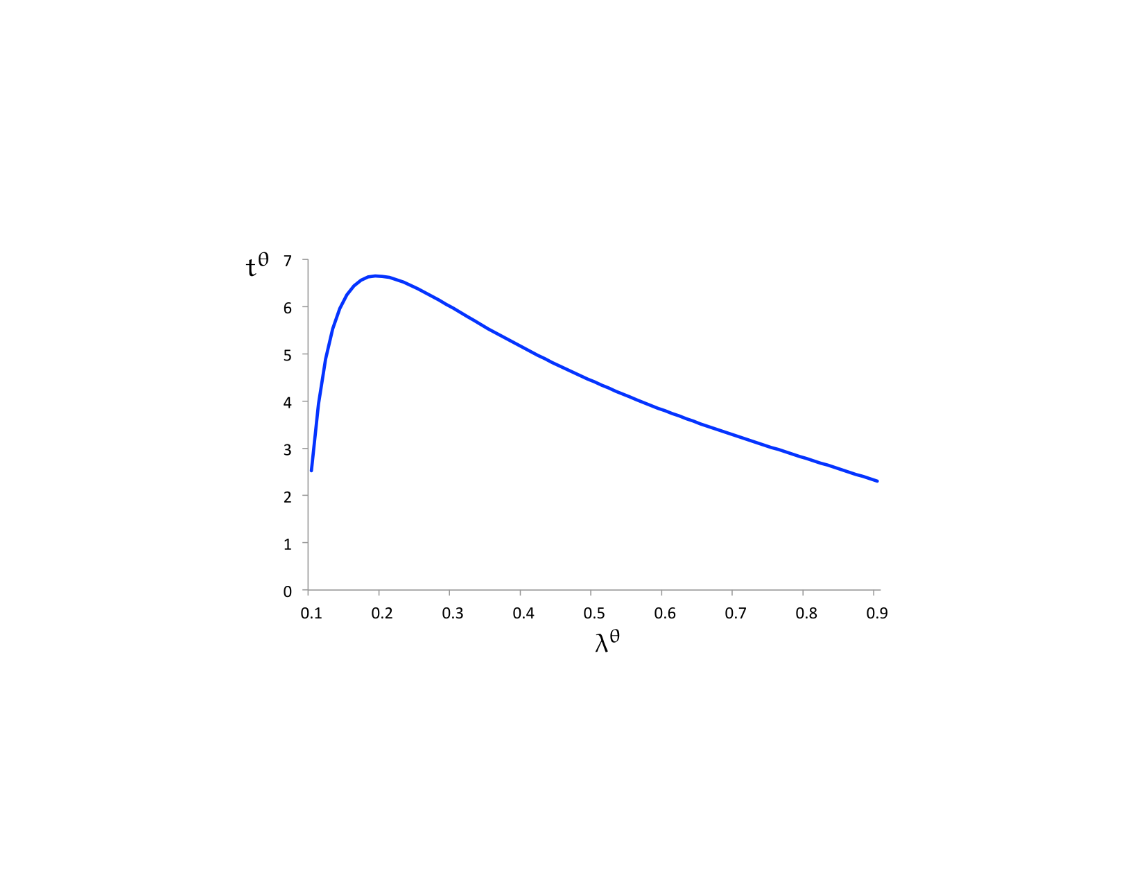
Equation (5) yields intuitive monotonicity of the first-best stopping time as a function of the prior that the project is good, $\beta_{0}$, and the cost of effort, $c$. But it also implies a fundamental non-monotonicity as a function of the agent’s ability, $\lambda^{\theta}$, as shown in Figure 1. (For simplicity, the figure ignores integer constraints on $t^{\theta}$.) This stems from the interaction of two countervailing forces. On the one hand, for any given belief about the state, the expected marginal benefit of effort is higher when the agent’s ability is higher; on the other hand, the higher is the agent’s ability, the more informative is a lack of success in a period in which he works. Hence, at any time $t>1$, a higher-ability agent is more pessimistic about the state (given that effort has been exerted in all prior periods), which has the effect of decreasing the expected marginal benefit of effort. Altogether, this makes the first-best stopping time non-monotonic in ability; both $t^{H}>t^{L}$ and $t^{H}<t^{L}$ are robust possibilities that arise for different parameters. As we will see, this has substantial implications.

Figure 1: The first-best stopping time.

The first-best expected discounted surplus at time zero from type $\theta$ is

$$\sum\limits_{t=1}^{t^{\theta}}\delta^{t}\left[\beta_{0}\left(1-\lambda^{\theta}\right)^{t-1}\left(\lambda^{\theta}-c\right)-(1-\beta_{0})c\right].$$

3.2 No adverse selection or no moral hazard

Our model has two sources of asymmetric information: adverse selection and moral hazard. To see that their interaction is essential, it is useful to understand what would happen in the absence of either one.

Consider first the case without adverse selection, i.e. assume the agent’s ability is observable but there is moral hazard. The principal can then use a constant-bonus contract to effectively sell the project to the agent at a price that extracts all the (ex-ante) surplus. Specifically, suppose the principal offers the agent of type $\theta$ a constant-bonus contract $\mathbf{C}^{\theta}=(t^{\theta},W^{\theta}_{0},1)$, where $W_{0}^{\theta}$ is chosen so that conditional on the agent exerting effort in each period up to the first-best termination date (as long as success has not obtained), the agent’s participation constraint at time zero binds:

$$U_{0}^{\theta}\left(\mathbf{C}^{\theta},\mathbf{1}\right)=\sum\limits_{t=1}^{t^{\theta}}\delta^{t}\left[\beta_{0}\left(1-\lambda^{\theta}\right)^{t-1}\left(\lambda^{\theta}-c\right)-(1-\beta_{0})c\right]+W_{0}^{\theta}=0,$$

where the notation $\mathbf{1}$ denotes the action profile of working in every period of the contract. Plainly, this contract makes the agent fully internalize the social value of success and hence achieves the first-best level of experimentation, while the principal keeps all the surplus.

Consider next the case with adverse selection but no moral hazard: the agent’s effort in any period still costs him $c>0$ but is observable and contractible. The principal can then implement the first best and extract all the surplus by using simple contracts that pay the agent for effort rather than outcomes. Specifically, the principal can offer the agent a choice between two contracts that involve no bonuses or penalties, with each paying the agent $c$ for every period that he works. The termination date is $t^{L}$ in the contract intended for the low type and $t^{H}$ in the contract intended for the high type. Plainly, the agent’s payoff is zero regardless of his type and which contract and effort profile he chooses. Hence, the agent is willing to choose the contract intended for his type and work until either a success is obtained or the termination date is reached.

To summarize:

Theorem 1.

If there is either no moral hazard or no adverse selection, the principal optimally implements the first best and extracts all the surplus.

A proof is omitted in light of the simple arguments preceding the theorem. Theorem 1 also holds when there are many types; that both kinds of information asymmetries are essential to generate distortions is general in our experimentation environment.

4 Second-Best (In)Efficiency

We now turn to the setting with both moral hazard and adverse selection. In this section, we formalize the principal’s problem and deduce the nature of second-best inefficiency. We provide explicit characterizations of optimal contracts in Section 5 and Section 6.

Without loss, we assume that the principal specifies a desired effort profile along with a contract. An optimal menu of contracts maximizes the principal’s ex-ante expected payoff subject to incentive compatibility constraints for effort (IC${}^{\theta}_{a}$ below), participation constraints (IR^θ below), and self-selection constraints for the agent’s choice of contract (IC${}^{\theta\theta^{\prime}}$ below). Denote

$$\bm{\alpha}^{\theta}\left(\mathbf{C}\right):=\operatorname*{arg\,max}\limits_{\mathbf{a}}\ U_{0}^{\theta}\left(\mathbf{C},\mathbf{a}\right)$$

as the set of optimal action plans for the agent of type $\theta$ under contract $\mathbf{C}$. With a slight abuse of notation, we will write $U^{\theta}_{0}(\mathbf{C},\bm{\alpha}^{\theta}(\mathbf{C}))$ for the type-$\theta$ agent’s utility at time zero from any contract $\mathbf{C}$. The principal’s program is:

$$\max_{\left(\mathbf{C}^{H},\mathbf{C}^{L},\mathbf{a}^{H},\mathbf{a}^{L}\right)}\mu_{0}\Pi_{0}^{H}\left(\mathbf{C}^{H},\mathbf{a}^{H}\right)+\left(1-\mu_{0}\right)\Pi_{0}^{L}\left(\mathbf{C}^{L},\mathbf{a}^{L}\right)$$

subject to, for all $\theta,\theta^{\prime}\in\left\{L,H\right\}$,

$$\mathbf{a}^{\theta} \in\bm{\alpha}^{\theta}(\mathbf{C}^{\theta}), {}^{\theta}_{a}$$ (IC)

$$U_{0}^{\theta}(\mathbf{C}^{\theta},\mathbf{a}^{\theta}) \geq 0,$$ (IR^θ)

$$U_{0}^{\theta}(\mathbf{C}^{\theta},\mathbf{a}^{\theta}) \geq U_{0}^{\theta}(\mathbf{C}^{\theta^{\prime}},\bm{\alpha}^{\theta}(\mathbf{C}^{\theta^{\prime}})). {}^{\theta\theta^{\prime}}$$ (IC)

Adverse selection is reflected in the self-selection constraints (IC${}^{\theta\theta^{\prime}}$), as is familiar. Moral hazard is reflected directly in the constraints (IC${}^{\theta}_{a}$) and also indirectly in the constraints (IC${}^{\theta\theta^{\prime}}$) via the term $\bm{\alpha}^{\theta}(\mathbf{C}^{\theta^{\prime}})$. To get a sense of how these matter, consider the agent’s incentive to work in some period $t$. This is shaped not only by the transfers that are directly tied to success/failure in period $t$ ($b_{t}$ and $l_{t}$) but also by the transfers tied to subsequent outcomes, through their effect on continuation values. In particular, ceteris paribus, raising the continuation value (say, by increasing either $b_{t+1}$ or $l_{t+1}$) makes reaching period $t+1$ more attractive and hence reduces the incentive to work in period $t$: this is a dynamic agency effect. Note moreover that the continuation value at any point in a contract depends on the agent’s type and his effort profile; hence it is not sufficient to consider a single continuation value at each period. Furthermore, besides having an effect on continuation values, the agent’s type also affects current incentives for effort because the expected marginal benefit of effort in any period differs for the two types. Altogether, the optimal plan of action will generally be different for the two types of the agent, i.e. for an arbitrary contract $\mathbf{C}$, we may have $\bm{\alpha}^{H}(\mathbf{C})\cap\bm{\alpha}^{L}(\mathbf{C})=\emptyset$.

Our result on second-best (in)efficiency is as follows:

Theorem 2.

In any optimal menu of contracts, each type $\theta\in\{L,H\}$ is induced to work for some number of periods, $\overline{t}^{\theta}$. Relative to the first-best stopping times, $t^{H}$ and $t^{L}$, the second best has $\overline{t}^{H}=t^{H}$ and $\overline{t}^{L}\leq t^{L}$.

Proof.

See Appendix A. ∎

Theorem 2 says that relative to the first best, there is no distortion in the amount of experimentation by the high-ability agent whereas the low-ability agent may be induced to under-experiment. It is interesting that this is a familiar “no distortion (only) at the top” result from static models of adverse selection, even though the inefficiency arises here from the conjunction of adverse selection and dynamic moral hazard (cf. Theorem 1). Moral hazard generates an “information rent” for the high type but not for the low type. As will be elaborated subsequently, reducing the low type’s amount of experimentation allows the principal to reduce the high type’s information rent. The optimal $\overline{t}^{L}$ trades off this information rent with the low type’s efficiency. For typical parameters, it will be the case that $\overline{t}^{L}\in\{1,\ldots,t^{L}-1\}$, so that the low type engages in some experimentation but not as much as socially efficient; however, it is possible that the low type is induced to not experiment at all ($\overline{t}^{L}=0$) or to experiment for the first-best amount of time ($\overline{t}^{L}=t^{L}$). The former possibility arises for reasons akin to exclusion in the standard model (e.g. the prior, $\mu_{0}$, on the high type is sufficiently high); the latter possibility is because time is discrete. Indeed, if the length of each time interval shrinks and one takes a suitable continuous-time limit, then there will be some distortion, i.e. $\overline{t}^{L}<t^{L}$.

The proof of Theorem 2 does not rely on characterizing second-best contracts. We establish $\overline{t}^{H}=t^{H}$ by proving that the low type’s self-selection constraint can always be satisfied without creating any distortions. The idea is that the principal can exploit the two types’ differing probabilities of success by making the high type’s contract “risky enough” to deter the low type from taking it, while still satisfying all other constraints. We establish $\overline{t}^{L}\leq t^{L}$ by showing that any contract for the low type inducing $\overline{t}^{L}>t^{L}$ can be modified by “removing” the last period of experimentation in this contract and concurrently reducing the information rent for the high type. Due to the lack of structure governing the high type’s behavior upon deviating to the low type’s contract, we prove the information-rent reduction no matter what action plan the high type would choose upon taking the low type’s contract. It follows that inducing over-experimentation by the low type cannot be optimal: not only would that reduce social surplus but it would also increase the high type’s information rent.

While Theorem 2 has implications for the extent of experimentation and innovation in different economic environments, we postpone such discussion to Subsection 5.3, after describing optimal contracts and their comparative statics.

5 Optimal Contracts when $t^{H}>t^{L}$

We characterize optimal contracts by first studying the case in which the first-best stopping times are ordered $t^{H}>t^{L}$, i.e. when the speed-of-learning effect that pushes the first-best stopping time down for a higher-ability agent does not dominate the productivity effect that pushes in the other direction. Any of the following conditions on the primitives is sufficient for $t^{H}>t^{L}$, given a set of other parameters: (i) $\beta_{0}$ is small enough, (ii) $\lambda^{L}$ and $\lambda^{H}$ are small enough, or (iii) $c$ is large enough. We maintain the assumption that $t^{H}>t^{L}$ implicitly throughout this section.

5.1 The solution

A class of solutions to the principal’s program described in Section 4 when $t^{H}>t^{L}$ is as follows:

Theorem 3.

Assume $t^{H}>t^{L}$. There is an optimal menu in which the principal separates the two types using penalty contracts. In particular, the optimum can be implemented using a onetime-penalty contract for type $H$, $\mathbf{C}^{H}=(t^{H},W^{H}_{0},l^{H}_{t^{H}})$ with $l^{H}_{t^{H}}<0<W^{H}_{0}$, and a penalty contract for type $L$, $\mathbf{C}^{L}=(\overline{t}^{L},W^{L}_{0},\bm{l}^{L})$, such that:

1. For all $t\in\{1,\ldots,\overline{t}^{L}\}$,

   $${l}_{t}^{L}=\begin{cases}-\left(1-\delta\right)\frac{c}{\overline{\beta}_{t}^{L}\lambda^{L}}&\text{ if }t<\overline{t}^{L}\text{,}\\ -\frac{c}{\overline{\beta}_{\overline{t}^{L}}^{L}\lambda^{L}}&\text{ if }t=\overline{t}^{L}\text{;}\end{cases}$$ (6)

2. $W^{L}_{0}>0$ is such that the participation constraint, (IR^L), binds;

3. Type $H$ gets an information rent: $U^{H}_{0}(\mathbf{C}^{H},\bm{\alpha}^{H}(\mathbf{C}^{H}))>0$;

4. $\mathbf{1}\in\bm{\alpha}^{H}(\mathbf{C}^{H})$; $\mathbf{1}\in\bm{\alpha}^{L}(\mathbf{C}^{L})$; and $\mathbf{1}=\bm{\alpha}^{H}(\mathbf{C}^{L})$.

Generically, the above contract is the unique optimal contract for type $L$ within the class of penalty contracts.

Proof.

See Appendix B. ∎

The optimal contract for the low type characterized by (6) is a penalty contract in which the magnitude of the penalty is increasing over time, with a “jump” in the contract’s final period. The jump highlights dynamic agency effects: by obtaining a success in a period $t$, the agent not only avoids the penalty $l^{L}_{t}$ but also the penalty $l^{L}_{t+1}$ and those after. The last period’s penalty needs to compensate for the absence of future penalties. Figure 2 depicts the low type’s contract; the comparative statics seen in the figure will be discussed subsequently. Only when there is no discounting does the low type’s contract reduce to a onetime-penalty contract where a penalty is paid only if the project has not succeeded by $\overline{t}^{L}$. For any discount factor, the high type’s contract characterized in Theorem 3 is a onetime-penalty contract in which he only pays a penalty to the principal if there is no success by the first-best stopping time $t^{H}$. On the equilibrium path, both types of the agent exert effort in every period until their respective stopping times; moreover, were the high type to take the low type’s contract (off the equilibrium path), he would also exert effort in every period of the contract. This implies that the high type gets an information rent because he would be less likely than the low type to incur any of the penalties in $\mathbf{C}^{L}$.

Although the optimal contract for the low type is (generically) unique among penalty contracts, there are a variety of optimal penalty contracts for the high type. The reason is that the low type’s optimal contract is pinned down by the need to simultaneously incentivize the low type’s effort and yet minimize the information rent obtained by the high type. This leads to a sequence of penalties for the low type, given by (6), that make him indifferent between working and shirking in each period of the contract, as we explain further in Subsection 5.2. On the other hand, the high type’s contract only needs to be made unattractive to the low type subject to incentivizing effort from the high type and providing the high type a utility level given by his information rent. There is latitude in how this can be done: the onetime penalty in the high type’s contract of Theorem 3 is chosen to be severe enough so that this contract is “too risky” for the low type to accept.

Remark 1.

The proof of Theorem 3 provides a simple algorithm to solve for an optimal menu of contracts. For any $\hat{t}\in\{0,\ldots,t^{L}\}$, we characterize an optimal menu that solves the principal’s program subject to an additional constraint that the low type must experiment until period $\hat{t}$. The low type’s contract in this menu is given by (6) with the termination date $\hat{t}$ rather than $\overline{t}^{L}$. An optimal (unconstrained) menu is then obtained by maximizing the principal’s objective function over $\hat{t}\in\{0,\ldots,t^{L}\}$.

The characterization in Theorem 3 yields the following comparative statics:

Proposition 2.

Assume $t^{H}>t^{L}$ and consider changes in parameters that preserve this ordering. The second-best stopping time for type $L$, $\overline{t}^{L}$, is weakly increasing in $\beta_{0}$ and $\lambda^{L}$, weakly decreasing in $c$ and $\mu_{0}$, and can increase or decrease in $\lambda^{H}$. The distortion in this stopping time, measured by $t^{L}-\overline{t}^{L}$, is weakly increasing in $\mu_{0}$ and can increase or decrease in $\beta_{0}$, $\lambda^{L}$, $\lambda^{H}$, and $c$.

Proof.

See the Supplementary Appendix. ∎

Figure 2 illustrates some of the conclusions of Proposition 2. The comparative static of $\overline{t}^{L}$ in $\mu_{0}$ is intuitive: the higher the ex-ante probability of the high type, the more the principal benefits from reducing the high type’s information rent and hence the more she shortens the low type’s experimentation. Matters are more subtle for other parameters. Consider, for example, an increase in $\beta_{0}$. On the one hand, this increases the social surplus from experimentation, which suggests that $\overline{t}^{L}$ should increase. But there are two other effects: holding fixed $\overline{t}^{L}$, penalties of lower magnitude can be used to incentivize effort from the low type because the project is more likely to succeed (cf. equation (6)), which has an effect of decreasing the information rent for the high type; yet, a higher $\beta_{0}$ also has a direct effect of increasing the information rent because the differing probability of success for the two types is only relevant when the project is good. Nevertheless, Proposition 2 establishes that it is optimal to (weakly) increase $\overline{t}^{L}$ when $\beta_{0}$ increases.

Since the high type’s information rent is increasing in $\lambda^{H}$, one may expect the principal to reduce the low type’s experimentation when $\lambda^{H}$ increases. However, a higher $\lambda^{H}$ means that the high type is likely to succeed earlier when deviating to the low type’s contract. For this reason, an increase in $\lambda^{H}$ can reduce the incremental information-rent cost of extending the low type’s contract, to the extent that the gain in efficiency from the low type makes it optimal to increase $\overline{t}^{L}$.

Figure 2: The optimal penalty contract for type $L$ under different values of $\mu_{0}$ and $\beta_{0}$. Both graphs have $\delta=0.5$, $\lambda^{L}=0.1$, $\lambda^{H}=0.12$, and $c=0.06$. The left graph has $\beta_{0}=0.89$, $\mu_{0}=0.3$, and $\mu_{0}^{\prime}=0.6$; the right graph has $\beta_{0}=0.85$, $\beta_{0}^{\prime}=0.89$, and $\mu_{0}=0.3$. The first-best entails $t^{L}=15$ on the left graph, and $t^{L}=12$ (for $\beta_{0}$) and $t^{L}=15$ (for $\beta^{\prime}_{0}$) on the right graph.

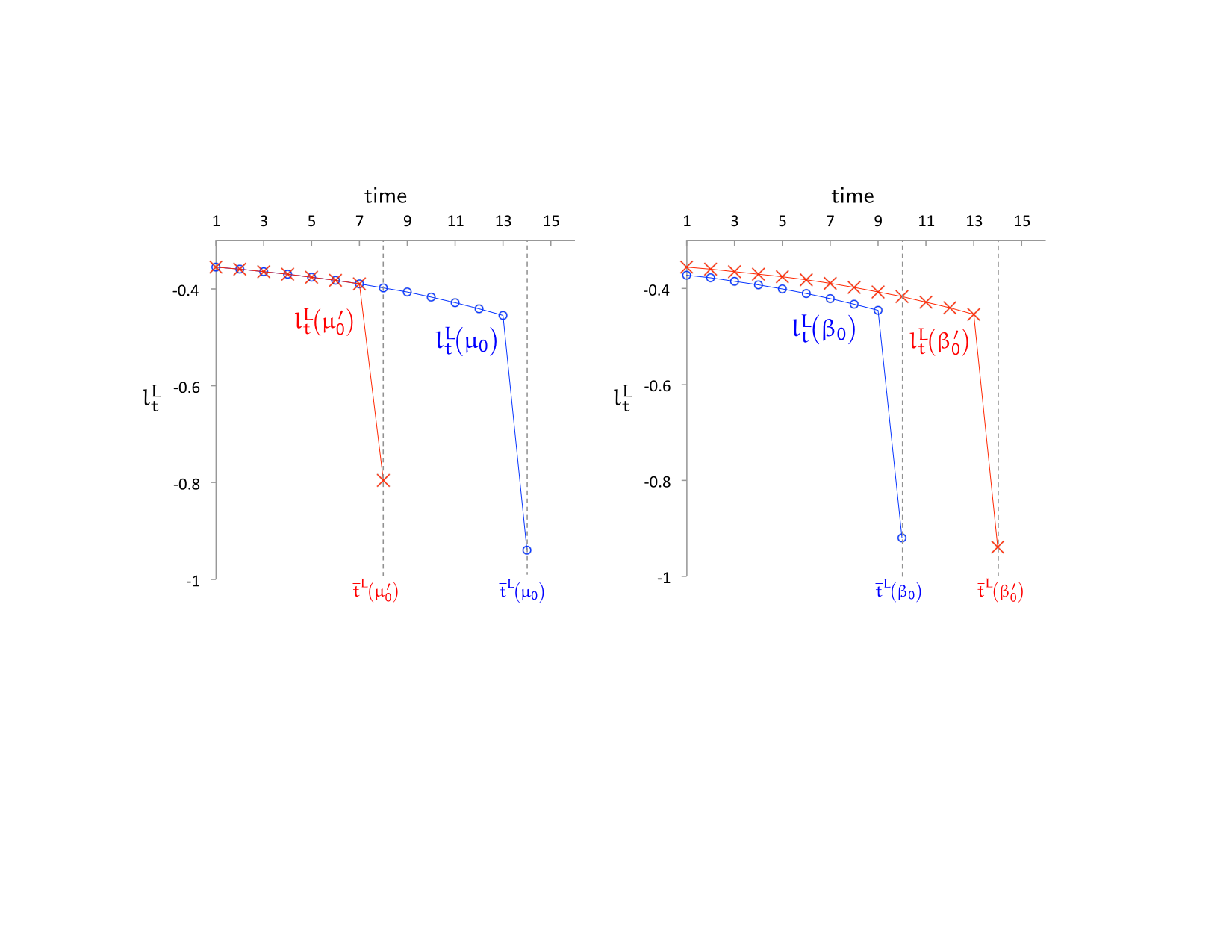
Turning to the magnitude of distortion, $t^{L}-\overline{t}^{L}$: since the first-best stopping time $t^{L}$ does not depend on the probability of a high type, $\mu_{0}$, while $\overline{t}^{L}$ is decreasing in this parameter, it is immediate that the distortion is increasing in $\mu_{0}$. The time $t^{L}$ is also independent of the high type’s ability, $\lambda^{H}$; thus, since $\overline{t}^{L}$ may increase or decrease in $\lambda^{H}$, the same is true for $t^{L}-\overline{t}^{L}$. Finally, with respect to $\beta_{0}$, $\lambda^{L}$, and $c$, the distortion’s ambiguous comparative statics stem from the fact that $t^{L}$ and $\overline{t}^{L}$ move in the same direction when these parameters change. For example, increasing $\beta_{0}$ can reduce $t^{L}-\overline{t}^{L}$ when $\mu_{0}$ is low but increase $t^{L}-\overline{t}^{L}$ when $\mu_{0}$ is high; the reason is that a larger ex-ante probability of the high type makes increasing $\overline{t}^{L}$ more costly in terms of information rent.

Theorem 3 utilizes penalty contracts in which the agent is required to pay the principal when he fails to obtain a success. While these contracts prove analytically convenient (as explained in Subsection 5.2), a weakness is that they do not satisfy interim participation constraints: in the implementation of Theorem 3, the agent of either type $\theta$ would “walk away” from his contract in any period $t\in\{1,\ldots,\overline{t}^{\theta}\}$ if he could. The following result provides a remedy:

Theorem 4.

Assume $t^{H}>t^{L}$. The second best can also be implemented using a menu of bonus contracts. Specifically, the principal offers type $L$ the bonus contract $\mathbf{C}^{L}=(\overline{t}^{L},W^{L}_{0},\bm{b}^{L})$ wherein for any $t\in\{1,\ldots,\overline{t}^{L}\}$,

$$b^{L}_{t}=\sum_{s=t}^{\overline{t}^{L}}\delta^{s-t}(-l_{s}^{L}),$$ (7)

where $\bm{l}^{L}$ is the penalty sequence in the optimal penalty contract given in Theorem 3, and $W^{L}_{0}$ is chosen to make the participation constraint, (IR^L), bind. For type $H$, the principal can use a constant-bonus contract $\mathbf{C}^{H}=(t^{H},W^{H}_{0},b^{H})$ with a suitably chosen $W^{H}_{0}$ and $b^{H}>0$.

Generically, the above contract is the unique optimal contract for type $L$ within the class of bonus contracts. This implementation satisfies interim participation constraints in each period for each type, i.e. each type $\theta$’s continuation utility at the beginning of any period $t\in\{1,\ldots,\overline{t}^{\theta}\}$ in $\mathbf{C}^{\theta}$ is non-negative.

A proof is omitted because the proof of Proposition 1 can be used to verify that each bonus contract in Theorem 4 is equivalent to the corresponding penalty contract in Theorem 3, and hence the optimality of those penalty contracts implies the optimality of these bonus contracts. Using (6), it is readily verified that in the bonus sequence (7),

$$b^{L}_{\overline{t}^{L}}=\frac{c}{\overline{\beta}^{L}_{\overline{t}^{L}}\lambda^{L}}\text{ and }b^{L}_{t}=\frac{(1-\delta)c}{\overline{\beta}^{L}_{t}\lambda^{L}}+\delta b^{L}_{t+1}\ \text{for any $t\in\{1,\ldots,\overline{t}^{L}-1\}$},$$ (8)

and hence the reward for success increases over time. When $\delta=1$, the low type’s bonus contract is a constant-bonus contract, analogous to the penalty contract in Theorem 3 being a onetime-penalty contract.

An interpretation of the bonus contracts in Theorem 4 is that the principal initially sells the project to the agent at some price (the up-front transfer $W_{0}$) with a commitment to buy back the output generated by a success at time-dated future prices (the bonuses $\bm{b}$).

5.2 Sketch of the proof

We now sketch in some detail how we prove Theorem 3. The arguments reveal how the interaction of adverse selection, dynamic moral hazard, and private learning jointly shape optimal contracts. This subsection also serves as a guide to follow the formal proof in Appendix B.

While we have defined a contract as $\mathbf{C}=(T,W_{0},\bm{b},\bm{l})$, it will be useful in this subsection alone (so as to parallel the formal proof) to consider a larger space of contracts, where a contract is given by $\mathbf{C}=\left(\Gamma,W_{0},\bm{b},\bm{l}\right)$. The first element here is a set of periods, $\Gamma\subseteq\mathbb{N}\setminus\{0\}$, at which the agent is not “locked out,” i.e. at which he is allowed to choose whether to work or shirk. As discussed in fn. 14, this additional instrument does not yield the principal any benefit, but it will be notationally convenient in the proof. The termination date of the contract is now $0$ if $\Gamma=\emptyset$ and otherwise $\max\Gamma$. We say that a contract is connected if $\Gamma=\{1,\ldots,T\}$ for some $T$; in this case we refer to $T$ as the length of the contract, and $T$ is also the termination date. The agent’s actions are denoted by $\mathbf{a}=\left(a_{t}\right)_{t\in\Gamma}$.

As justified by Proposition 1, we solve the principal’s problem (stated at the outset of Section 4) by restricting attention to menus of penalty contracts: for each $\theta\in\{L,H\}$, $\mathbf{C}^{\theta}=(\Gamma^{\theta},W^{\theta}_{0},\bm{l}^{\theta})$. Penalty contracts are analytically convenient to deal with the combination of adverse selection and dynamic moral hazard for reasons explained in Step 4 below.

Step 1: We simplify the principal’s program by (i) focussing on contracts for type $L$ that induce him to work in every non-lockout period, i.e. on contracts in the set $\{\mathbf{C}^{L}:\mathbf{1}\in\bm{\alpha}^{L}(\mathbf{C}^{L})\}$; and (ii) ignoring the constraints (IR^H) and (IC^LH). It is established in the proof of Theorem 2 that a solution to this simplified program also solves the original program. Call this program [P1].

It is not obvious a priori what action plan the high type may use when taking the low type’s contract. Accordingly, we tackle a relaxed program, [RP1], that replaces (IC^HL) in program [P1] by a relaxed version, called (Weak-IC^HL), that only requires type $H$ to prefer taking his contract and following an optimal action plan over taking type $L$’s contract and working in every period. Formally, (IC^HL) requires $U_{0}^{H}(\mathbf{C}^{H},\bm{\alpha}^{H}(\mathbf{C}^{H}))\geq U_{0}^{H}(\mathbf{C}^{L},\bm{\alpha}^{H}(\mathbf{C}^{L}))$ whereas (Weak-IC^HL) requires only $U_{0}^{H}(\mathbf{C}^{H},\bm{\alpha}^{H}(\mathbf{C}^{H}))\geq U_{0}^{H}(\mathbf{C}^{L},\mathbf{1})$. We emphasize that this restriction on type $H$’s action plan under type $L$’s contract is not without loss for an arbitrary contract $\mathbf{C}^{L}$; i.e., given an arbitrary $\mathbf{C}^{L}$ with $\mathbf{1}\in\bm{\alpha}^{L}(\mathbf{C}^{L})$, it need not be the case that $\mathbf{1}\in\bm{\alpha}^{H}(\mathbf{C}^{L})$—it is in this sense that there is no “single-crossing property” in general. The reason is that because of their differing probabilities of success from working in future periods (conditional on the good state), the two types trade off current and future penalties differently when considering exerting effort in the current period. In particular, the desire to avoid future penalties provides more of an incentive for the low type to work in the current period than the high type.

Relaxing (IC^HL) to (Weak-IC^HL) is motivated by a conjecture that even though the high type may choose to work less than the low type in an arbitrary contract, this will not be the case in an optimal contract for the low type. This relaxation is a critical step in making the program tractable because it severs the knot in the fixed point problem of optimizing over the low type’s contract while not knowing what action plan the high type would follow should he take this contract. The relaxation works because of the efficiency ordering $t^{H}>t^{L}$, as elaborated subsequently.

In the relaxed program [RP1], it is straightforward to show that (Weak-IC^HL) and (IR^L) must bind at an optimum: otherwise, time-zero transfers in one of the two contracts can be profitably lowered without violating any of the constraints. Consequently, one can substitute from the binding version of these constraints to rewrite the objective function as the sum of total surplus less an information rent for the high type, as in the standard approach. We are left with a relaxed program, [RP2], which maximizes this objective function and whose only constraints are the direct moral hazard constraints (IC${}_{a}^{H}$) and (IC${}_{a}^{L}$), where type $L$ must work in all periods. This program is tractable because it can be solved by separately optimizing over each type’s penalty contract. The following steps 2–5 derive an optimal contract for type $L$ in program [RP2] that has useful properties.

Step 2: We show that there is an optimal penalty contract for type $L$ that is connected. A rough intuition is as follows. Because type $L$ is required to work in all non-lockout periods, the value of the objective function in program [RP2] can be improved by removing any lockout periods in one of two ways: either by “shifting up” the sequence of effort and penalties or by terminating the contract early (suitably adjusting for discounting in either case). Shifting up the sequence of effort and penalties eliminates inefficient delays in type $L$’s experimentation, but it also increases the rent given to type $H$, because the penalties—which are more likely to be borne by type $L$ than type $H$—are now paid earlier. Conversely, terminating the contract early reduces the rent given to type $H$ by lowering the total penalties in the contract, but it also shortens experimentation by type $L$. It turns out that either of these modifications may be beneficial to the principal, but at least one of them will be if the initial contract is not connected.

Step 3: Given any termination date $T^{L}$, there are many penalty sequences that can be used by a connected penalty contract of length $T^{L}$ to induce the low-ability agent to work in each period $1,\ldots,T^{L}$. We construct the unique sequence, call it $\overline{\bm{l}}(T^{L})$, that ensures the low type’s incentive constraint for effort binds in each period of the contract, i.e. in any period $t\in\{1,\ldots,T^{L}\}$, the low type is indifferent between working (and then choosing any optimal effort profile in subsequent periods) and shirking (and then choosing any optimal effort profile in subsequent periods), given the past history of effort. The intuition is straightforward: in the final period, $T^{L}$, there is obviously a unique such penalty as it must solve $\overline{l}^{L}_{T^{L}}(T^{L})=-c+(1-\overline{\beta}^{L}_{T^{L}}\lambda^{L})\overline{l}^{L}_{T^{L}}(T^{L})$. Iteratively working backward using a one-step deviation principle, this pins down penalties in each earlier period through the (forward-looking) incentive constraint for effort in each period. Naturally, for any $T^{L}$ and $t\in\{1,\ldots,T^{L}\}$, $\overline{l}^{L}_{t}(T^{L})<0$, i.e. as suggested by the term “penalty”, the agent pays the principal each time there is a failure.

Step 4: We show that any connected penalty contract for type $L$ that solves program [RP2] must use the penalty structure $\overline{\bm{l}}^{L}(\cdot)$ of Step 3. The idea is that any slack in the low type’s incentive constraint for effort in any period can be used to modify the contract to strictly reduce the high type’s expected payoff from taking the low type’s contract (without affecting the low type’s behavior or expected payoff), based on the high type succeeding with higher probability in every period when taking the low type’s contract.

Although this logic is intuitive, a formal argument must deal with the challenge that modifying a transfer in any period to reduce slack in the low type’s incentive constraint for effort in that period has feedback on incentives in every prior period—the dynamic agency problem. Our focus on penalty contracts facilitates the analysis here because penalty contracts have the property that reducing the incentive to exert effort in any period $t$ by decreasing the severity of the penalty in period $t$ has a positive feedback of also reducing the incentive for effort in earlier periods, since the continuation value of reaching period $t$ increases. Due to this positive feedback, we are able to show that the low type’s incentive for effort in a given period of a connected penalty contract can be modified without affecting his incentives in any other period by solely adjusting the penalties in that period and the previous one. In particular, in an arbitrary connected penalty contract $\mathbf{C}^{L}$, if type $L$’s incentive constraint is slack in some period $t$, we can increase $l^{L}_{t}$ and reduce $l^{L}_{t-1}$ in a way that leaves type $L$’s incentives for effort unchanged in every period $s\neq t$ while still being satisfied in period $t$. We then verify that this “local modification” strictly reduces the high type’s information rent.

Step 5: In light of Steps 2–4, all optimal connected penalty contracts for type $L$ in program [RP2] can be found by just optimizing over the length of connected penalty contracts with the penalty structure $\overline{\bm{l}}^{L}(\cdot)$. By Theorem 2, the optimal length, $\overline{t}^{L}$, cannot be larger than the first-best stopping time: $\overline{t}^{L}\leq t^{L}$. In this step, we further establish that $\overline{t}^{L}$ is generically unique, and that generically there is no optimal penalty contract for type $L$ that is not connected.

Step 6: Let $\overline{\mathbf{C}}^{L}$ be the contract for type $L$ identified in Steps 2–5. Recall that [RP1] differs from the principal’s original program [P1] in that it imposes (Weak-IC^HL) rather than (IC^HL). In this step, we show that any solution to [RP1] using $\overline{\mathbf{C}}^{L}$ satisfies (IC^HL) and hence is also a solution to program [P1]. Specifically, we show that $\bm{\alpha}^{H}(\overline{\mathbf{C}}^{L})=\mathbf{1}$, i.e. if type $H$ were to take contract $\overline{\mathbf{C}}^{L}$, it would be uniquely optimal for him to work in all periods $1,\ldots,\overline{t}^{L}$. The intuition is as follows: under contract $\overline{\mathbf{C}}^{L}$, type $H$ has a higher expected probability of success from working in any period $t\leq\overline{t}^{L}$, no matter his prior choices of effort, than does type $L$ in period $t$ given that type $L$ has exerted effort in all prior periods (recall $\mathbf{1}\in\bm{\alpha}^{L}(\overline{\mathbf{C}}^{L})$). The argument relies on Theorem 2 having established that $\overline{t}^{L}\leq t^{L}$, because $t^{H}>t^{L}$ then implies that for any $t\in\{1,\ldots,\overline{t}^{L}\}$, $\beta^{H}_{t}\lambda^{H}>\overline{\beta}^{L}_{t}\lambda^{L}$ for any history of effort by type $H$ in periods $1,\ldots,t-1$. Using this property, we verify that because $\overline{\mathbf{C}}^{L}$ makes type $L$ indifferent between working and shirking in each period up to $\overline{t}^{L}$ (given that he has worked in all prior periods), type $H$ would find it strictly optimal to work in each period up to $\overline{t}^{L}$ no matter his prior history of effort.

5.3 Implications and applications

Asymmetric information and success.

Our results offer predictions on the extent of experimentation and innovation. An immediate implication concerns the effects of asymmetric information. Compare a setting with either no moral hazard or no adverse selection, as in Theorem 1, with a setting where both features are present, as in Theorem 2. The theorems reveal that, other things equal, the amount of experimentation will be lower in the latter, and, consequently, the average probability of success will also be lower. Furthermore, because low-ability agents’ experimentation is typically distorted down whereas that of high-ability agents is not, we predict a larger dispersion in success rates across agents and projects when both forms of asymmetric information are present.

Our analysis also bears on the relationship between innovation rates and the quality of the underlying environment. Absent any distortions, “better environments” lead to more success. In particular, an increase in the agent’s average ability, $\mu_{0}\lambda^{H}+(1-\mu_{0})\lambda^{L}$, yields a higher probability of success in the first best. However, contracts designed in the presence of moral hazard and adverse selection need not produce this property. The reason is that an improvement in the agent’s average ability can make it optimal for the principal to distort experimentation by more: as shown in Proposition 2, $\overline{t}^{L}$ decreases in $\mu_{0}$ and, for some parameter values, in $\lambda^{H}$. Such a reduction in $\overline{t}^{L}$ can decrease the second-best average success probability when the agent’s average ability increases. Consequently, observing higher innovation rates in contractual settings is neither necessary nor sufficient to deduce a better underlying environment.

Contract farming and technology adoption.

Though our model is not developed to explain a particular application, our framework speaks to contract farming and, more broadly, technology adoption in developing countries. Technology adoption is inherently a dynamic process of experimentation and learning. Understanding the adoption of agricultural innovations in low-income countries, and the obstacles to it, has been a central topic in development economics (Feder, Just, and Zilberman, 1985; Foster and Rosenzweig, 2010). Practitioners, policymakers, and researchers have long recognized the importance of contractual arrangements to provide proper incentives, because farmers typically don’t internalize the broader benefits of their experimentation.

As described in the Introduction, contract farming is a common practice in developing countries; it involves a profit-maximizing firm, which is typically a large-scale buyer such as an exporter or a food processor, and a farmer, who may be a small or a large grower. The contractual environment features not only learning about the quality of new seeds or a new technology, but also moral hazard and unobservable heterogeneity (Miyata et al., 2009). The arrangements used between agricultural firms and farmers resemble the contracts characterized in Theorem 4, with firms committing to time-dated future prices for an output of a certain quality delivered by a given deadline. Our analysis shows why such contracts are optimal in the presence of uncertainty, moral hazard, and unobservable heterogeneity, and how the shape of the contract hinges on the interaction of these three key features. Theorem 4 and formula (8) reveal how an optimal pattern of outcome-contingent buyback prices should be determined. In principle, these predicted contracts could be subject to empirical testing.

Much of the recent research on technology adoption uses controlled field experiments to study the incentives of potential adopters. Our results may inform the design of experimental work, particularly with regards to dynamic considerations, which are receiving increasing attention. For example, Jack et al. (2014) use a field experiment to study both the initial take-up decision and the subsequent investment (follow-through) decisions in the context of agricultural technology (tree species) adoption in Zambia. The authors consider simple contracts to investigate the interplay between the uncertainty of a technology’s profitability, the self-selection of farmers, and learning of new information. In their experimental design, contracts specify the initial price of the technology and an outcome-contingent payment tied to the survival of trees by the end of one year. The study uses variation of the contracts in the two dimensions (initial price and contingent payment) to evaluate their performance. The authors find that 35% of farmers who pay a positive price for take-up have no trees one year later; in addition, among farmers who follow-through, the tree survival rate responds to learning over time.

The contract form used in Jack et al. (2014) shares features with what emerges as an optimal contract in our model, and their basic findings are also consistent with our results. Their controlled experiment is simple in that performance is assessed and a reward is paid only at the end of one year. Our model shows that to optimally incentivize experimentation, agents must be compensated with continual rewards contingent on the time of success, up until an optimally chosen termination date which may differ from the efficient stopping time. Moreover, perhaps counterintuitively, Theorem 4 shows that higher rewards must be offered for later success, with the rate of increase depending on the rate of learning (and other factors). Our results thus point to a new dimension that can improve follow-through rates; this could be tested in future field experiments.

Finally, many scholars study the puzzle of low technology adoption rates and its potential solutions (e.g., Suri, 2011, and the references therein). Our paper adds to the discussion by relating adoption rates to the underlying contractual environment. As mentioned earlier, we predict less experimentation, lower success rates, and more dispersion of success rates in settings with more asymmetric information; the lower (and more dispersed) success rates translate into lower (and more dispersed) adoption rates. We also find that the relationship between adoption rates and the underlying environment can be subtle, with “better environments” possibly leading to less experimentation and lower adoption in the second best. Our results thus provide a novel explanation for the low adoption rate puzzle. Empirical researchers have recently been interested in how agency contributes to the puzzle (e.g., Atkin et al., 2015); our work contributes to the theoretical background for such lines of inquiry.

Naturally, there are dimensions of contract farming and technology adoption that our analysis does not cover. For example, social learning among farmers affects adoption (Conley and Udry, 2010), and agricultural companies will want to take this into account when designing contracts. A deeper understanding of optimal contracts for multiple experimenting agents who can learn from each other would be useful for this application. While this and similar extensions may yield new insights, we expect our main results to be robust: to reduce the information rent of high-ability types, the principal will benefit from distorting the length of experimentation of low-ability types, and from setting payments so that their incentive constraint for effort binds at each time. This suggests that, under appropriate conditions, an agent will still receive a higher reward for succeeding later rather than earlier.

Book contracts.

As mentioned in the Introduction, some contractual relationships between a publisher and author have the features we study: it is initially uncertain whether a satisfactory book can be written in the relevant timeframe; the author may be privately informed about his suitability for the task; and how much time the author spends on this is not observable to the publisher. It is common for real-world publishing contracts to resemble the penalty contracts characterized in Theorem 3: book contracts pay an advance to the author that the publisher can recoup if the author fails to deliver on time (according to a delivery-of-manuscript clause) or if the book is unacceptable (according to a satisfactory-manuscript clause); see Bunnin (1983) and Fowler (1985). There is substantial dispersion in both the deadlines and the advances that authors are given; Kuzyk,Raya (2006) notes that publishing houses try to assess an author’s chances of succeeding when determining these terms.

6 Optimal Contracts when $t^{H}\leq t^{L}$

We now turn to characterizing optimal contracts when the first-best stopping times are ordered $t^{H}\leq t^{L}$. Any of the following conditions on the primitives is sufficient for this case given a set of other parameters: (i) $\beta_{0}$ is large enough, (ii) $\lambda^{H}$ is large enough, or (iii) $c$ is small enough.

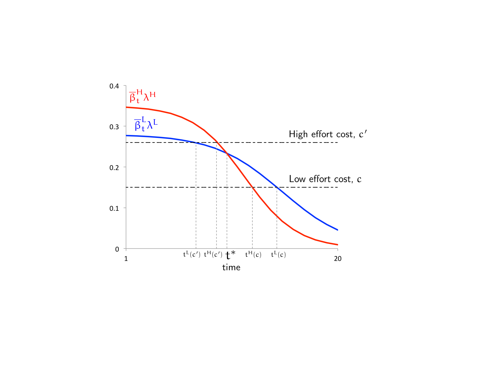
The principal’s program remains as described in Section 4, but solving the program is now substantially more difficult than when $t^{H}>t^{L}$. To understand why, consider Figure 3, which depicts the two types’ “no-shirk expected marginal product” curves, $\overline{\beta}^{\theta}_{t}\lambda^{\theta}$, as a function of time. (For simplicity, the figure is drawn ignoring integer constraints.) For any parameters, these curves cross exactly once as shown in the figure; the crossing point $t^{*}$ is the unique solution to

$$\mbox{$\overline{\beta}^{H}_{t^{*}}\lambda^{H}-\overline{\beta}^{L}_{t^{*}}\lambda^{L}\geq 0>\overline{\beta}^{H}_{t^{*}+1}\lambda^{H}-\overline{\beta}^{L}_{t^{*}+1}\lambda^{L}$}.$$

Parameters under which $t^{H}>t^{L}$ entail $t^{L}<t^{*}$, as seen with the high effort cost in Figure 3. When $t^{L}\leq t^{*}$, it holds at any $t\leq t^{L}$ that the high type has a higher expected marginal product than the low type conditional on the agent working in all prior periods. It is this fact that allowed us to prove Theorem 3 by conjecturing that the high type would work in every period when taking the low type’s contract.

By contrast, $t^{H}\leq t^{L}$ implies $t^{L}\geq t^{*}$, as seen with the low effort cost in Figure 3. Since the second-best stopping time for the low type can be arbitrarily close to his first-best stopping time (e.g. if the prior on the low type, $1-\mu_{0}$, is sufficiently large), it is no longer valid to conjecture that the high type will work in every period when taking the low type’s optimal contract—in this sense, “single crossing” need not hold even at the optimum. The reason is that at some period after $t^{*}$, given that both types have worked in each prior period, the high type can be sufficiently more pessimistic than the low type that the high type finds it optimal to shirk in some or all of the remaining periods, even though $\lambda^{H}>\lambda^{L}$ and the low type would be willing to work for the contract’s duration. Indeed, this will necessarily be true in the last period of the low type’s contract if this period is later than $t^{*}$ and the contract makes the low type just indifferent between working and shirking in this period as in the characterization of Theorem 3.

Figure 3: No-shirk expected marginal product curves with $\beta_{0}=0.99,\lambda^{L}=0.28,\lambda^{H}=0.35$.

Solving the principal’s program without being able to restrict attention to some suitable subset of action plans for the high type when he takes the low type’s contract appears intractable. For an arbitrary $\delta$, we have been unable to find a valid restriction. The following example elucidates the difficulties.

Example 1.

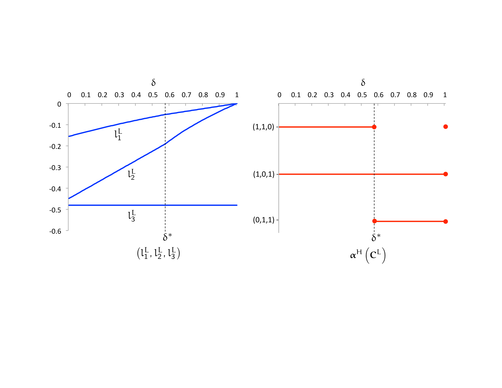
For an open and dense set of parameters $\{\beta_{0},c,\lambda^{L},\lambda^{H}\}$ with $\overline{t}^{L}=t^{L}=3$, there is a $\delta^{*}\in(0,1)$ such that the optimal penalty contract for type $L$ as a function of the discount factor, $\mathbf{C}^{L}(\delta)=(3,W^{L}_{0}(\delta),\bm{l}^{L}(\delta))$, has the property that the optimal action plans for type $H$ under this contract are given by

$$\bm{\alpha}^{H}(\mathbf{C}^{L}(\delta))=\begin{cases}\{(1,1,0),(1,0,1)\}&\mbox{if }\delta\in(0,\delta^{*})\\ \{(1,1,0),(1,0,1),(0,1,1)\}&\mbox{if }\delta=\delta^{*}\\ \{(1,0,1),(0,1,1)\}&\mbox{if }\delta\in(\delta^{*},1)\\ \{(1,1,0),(1,0,1),(0,1,1)\}&\mbox{if }\delta=1.\\ \end{cases}$$

Figure 4 depicts the contract and type $H$’s optimal action plans as a function of $\delta$ for a particular set of other parameters. Notice that the only action plan that is optimal for type $H$ for all $\delta$ is the non-consecutive-work plan $(1,0,1)$, but for each value of $\delta$ at least one other plan is also optimal. Interestingly, the stopping strategy $(1,1,0)$ is not optimal for type $H$ when $\delta\in(\delta^{*},1)$ although it is when $\delta=1$. The lack of lower hemi-continuity of $\bm{\alpha}^{H}(\mathbf{C}^{L}(\delta))$ at $\delta=1$ is not an accident, as we will discuss subsequently.

Figure 4: The optimal penalty contract for type $L$ in Example 1 with $\beta_{0}=0.86$, $c=0.1$, $\lambda^{L}=0.75$, $\lambda^{H}=0.95$ (left graph) and the optimal action profiles for type $H$ under this contract (right graph).

Nevertheless, we are able to solve the problem when $\delta=1$.

Theorem 5.

Assume $\delta=1$ and $t^{H}\leq t^{L}$. There is an optimal menu in which the principal separates the two types using onetime-penalty contracts, $\mathbf{C}^{H}=(t^{H},W^{H}_{0},l^{H}_{t^{H}})$ with $l^{H}_{t^{H}}<0<W^{H}_{0}$ for type $H$ and $\mathbf{C}^{L}=(\overline{t}^{L},W^{L}_{0},l^{L}_{\overline{t}^{L}})$ for type $L$, such that:

1. $l^{L}_{\overline{t}^{L}}=\min\left\{-\frac{c}{\overline{\beta}^{L}_{\overline{t}^{L}}\lambda^{L}},-\frac{c}{\overline{\beta}^{H}_{t^{HL}}\lambda^{H}}\right\}$, where $t^{HL}:=\max\limits_{\mathbf{a}\in\bm{\alpha}^{H}\left(\mathbf{C}^{L}\right)}\#\left\{n:a_{n}=1\right\}$;

2. $W^{L}_{0}>0$ is such that the participation constraint, (IR^L), binds;

3. Type $H$ gets an information rent: $U^{H}_{0}(\mathbf{C}^{H},\bm{\alpha}^{H}(\mathbf{C}^{H}))>0$;

4. $\mathbf{1}\in\bm{\alpha}^{H}(\mathbf{C}^{H})$; $\mathbf{1}\in\bm{\alpha}^{L}(\mathbf{C}^{L})$.

Proof.

See Appendix C. ∎

For $\delta=1$, the optimal menus of penalty contracts characterized in Theorem 5 for $t^{H}\leq t^{L}$ share some common properties with those characterized in Theorem 3 for $t^{H}>t^{L}$: in both cases, a onetime-penalty contract is used for the low type and the high type earns an information rent. On the other hand, part 1 of Theorem 5 points to two differences: (i) it will generally be the case in the optimal $\mathbf{C}^{L}$ that when $t^{H}\leq t^{L}$, $\mathbf{1}\notin\bm{\alpha}^{H}(\mathbf{C}^{L})$, whereas for $t^{H}>t^{L}$, $\bm{\alpha}^{H}(\mathbf{C}^{L})=\mathbf{1}$; and (ii) when $t^{H}\leq t^{L}$, it can be optimal for the principal to induce the low type to work in each period by satisfying the low type’s incentive constraint for effort with slack (i.e. with strict inequality), whereas when $t^{H}>t^{L}$, the penalty sequence makes this effort constraint bind in each period.

The intuition for these differences derives from information rent minimization considerations. The high type earns an information rent because by following the same effort profile as the low type he is less likely to incur any penalty for failure, and hence has a higher utility from any penalty contract than the low type. Minimizing the rent through this channel suggests minimizing the magnitude of the penalties that are used to incentivize the low type’s effort; it is this logic that drives Theorem 3 and for $\delta=1$ leads to a onetime-penalty contract with

$$l^{L}_{\overline{t}^{L}}=-\frac{c}{\overline{\beta}^{L}_{\overline{t}^{L}}\lambda^{L}}.$$ (9)

However, when $\overline{t}^{L}>t^{*}$ (which is only possible when $t^{H}\leq t^{L}$), the high type would find it optimal under this contract to work only for some $T<\overline{t}^{L}$ number of periods. It is then possible—and is true for an open and dense set of parameters—that $T$ is such that the high type is more likely to incur the onetime penalty than the low type. But in such a case, the penalty given in (9) would not be optimal because the principal can lower $l^{L}_{\overline{t}^{L}}$ (i.e. increase the magnitude of the penalty) to reduce the information rent, which she can keep doing until the high type finds it optimal to work for more periods and becomes less likely to incur the onetime penalty than the low type. This explains part 1 of Theorem 5.

We should note that this possibility arises because time is discrete. It can be shown that when the length of time intervals vanishes, in real-time the $t^{HL}$ and $\overline{t}^{L}$ in the statement of Theorem 5 are such that $\overline{\beta}^{L}_{\overline{t}^{L}}\lambda^{L}\leq\overline{\beta}^{H}_{t^{HL}}\lambda^{H}$ (in particular, $\overline{\beta}^{L}_{\overline{t}^{L}}\lambda^{L}=\overline{\beta}^{H}_{t^{HL}}\lambda^{H}$ when $\overline{t}^{L}>t^{HL}$, or equivalently when $\overline{t}^{L}>t^{*}$), and hence $l^{L}_{\overline{t}^{L}}=-\frac{c}{\overline{\beta}^{L}_{\overline{t}^{L}}\lambda^{L}}$ is optimal, just as in Theorem 3 when $\delta=1$. Intuitively, because learning is smooth in continuous time, the high type would always work long enough upon deviating to the low type’s contract that he is less likely to incur the onetime penalty $l^{L}_{\overline{t}^{L}}$ than the low type. Thus, by the logic above, lowering the onetime penalty below that in (9) would only increase the information rent of the high type in the continuous-time limit.

Remark 2.

The proof of Theorem 5 provides an algorithm to solve for an optimal menu of contracts when $t^{H}\leq t^{L}$ and $\delta=1$. For each pair of integers $(s,t)$ such that $0\leq s\leq t\leq t^{L}$, one can compute the principal’s payoff from using the onetime-penalty contract for type $L$ given by Theorem 5 when $\overline{t}^{L}$ is replaced by $t$ and $t^{HL}$ is replaced by $s$. Optimizing over $(s,t)$ then yields an optimal (unconstrained) menu.

How do we prove Theorem 5 in light of the difficulties described earlier of finding a suitable restriction on the high type’s behavior when taking the low-type’s contract? The answer is that when $\delta=1$, one can conjecture that the optimal contract for the low type must be a onetime-penalty contract (as was also true when $t^{H}>t^{L}$). Notice that because of no discounting, any onetime-penalty contract would make the agent of either type indifferent among all action plans that involve the same number of periods of work. In particular, a stopping strategy—an action plan that involves consecutive work for some number of periods followed by shirking thereafter—is always optimal for either type in a onetime-penalty contract. The heart of the proof of Theorem 5 establishes that it is without loss of generality to restrict attention to penalty contracts for the low type under which the high type would find it optimal to use a stopping strategy (see Subsection C.4 in Appendix C). With this in hand, we are then able to show that a onetime-penalty contract for the low type is indeed optimal (see Subsection C.5). Finally, the rent-minimization considerations described above are used to complete the argument. Observe that optimality of a onetime-penalty contract for the low type and that of a stopping strategy for the high type under such a contract is consistent with the solution in Example 1 for $\delta=1$, as seen in Figure 4. Moreover, the example plainly shows that such a strategy space restriction will not generally be valid when $\delta<1$.

We provide a bonus-contracts implementation of Theorem 5:

Theorem 6.

Assume $\delta=1$ and $t^{H}\leq t^{L}$. The second-best can also be implemented using a menu of constant-bonus contracts: $\mathbf{C}^{L}=(\overline{t}^{L},W^{L}_{0},b^{L})$ with $b^{L}=-l^{L}_{\overline{t}^{L}}>0>W^{L}_{0}$ where $l^{L}_{\overline{t}^{L}}$ is given in Theorem 5, and $\mathbf{C}^{H}=(t^{H},W^{H}_{0},b^{H})$ with a suitably chosen $W^{H}_{0}$ and $b^{H}>0$.

A proof is omitted since this result follows directly from Theorem 5 and the proof of Proposition 1 (using $\delta=1$). For similar reasons to those discussed around Theorem 4, the implementation in Theorem 6 satisfies interim participation constraints whereas that of Theorem 5 does not.

We end this section by emphasizing that although we are unable to characterize second-best optimal contracts when $\delta<1$ and $t^{H}\leq t^{L}$, the (in)efficiency conclusions from Theorem 2 apply for all parameters.

7 Discussion

7.1 Private observability and disclosure

Suppose that project success is privately observed by the agent but can be verifiably disclosed. The principal’s payoff from project success obtains here only when the agent discloses it, and contracts are conditioned not on project success but rather the disclosure of project success. Private observability introduces additional constraints for the principal because the agent must also now be incentivized to not withhold project success. For example, in a bonus contract where $\delta b_{t+1}>b_{t}$, an agent who obtains success in period $t$ would strictly prefer to withhold it and continue to period $t+1$, shirk in that period, and then reveal the success at the end of period $t+1$. Nevertheless, we show in the Supplementary Appendix that private observability does not reduce the principal’s payoff compared to our baseline setting: in each of the menus identified in Theorems 3–6, each of the contracts would induce the agent (of either type) to reveal project success immediately when it is obtained, so these menus remain optimal and implement the same outcome as when project success is publicly observable.

7.2 Limited liability

To focus on the interaction of adverse selection and moral hazard in experimentation, we have abstracted away from limited-liability considerations. Consider introducing the requirement that all transfers must be above some minimum threshold, say zero. The Supplementary Appendix shows how such a limited-liability constraint alters the second-best solution for the case of $t^{H}>t^{L}$ and $\delta=1$. This constraint results in both types of the agent acquiring a rent, so long as they are both induced to experiment. Three points are worth emphasizing. First, each type’s second-best stopping time is no larger than his first-best stopping time. The logic precluding over-experimentation, however, is somewhat different—and simpler—than without limited liability: inducing over-experimentation requires paying a bonus of more than one (the principal’s value of success) in the last period of the contract in which the agent works, implying a loss for the principal which under limited liability cannot be offset through an up-front payment. Second, while both types’ second-best stopping times are now (typically) distorted, their ordering is the same as without limited liability (i.e., $\overline{t}^{L}\leq\overline{t}^{H}$). The reason is that the principal could otherwise improve upon the menu by just offering both types the low type’s contract, which would induce the high type to experiment longer without increasing the high type’s payoff. Third, the principal can implement the second-best stopping time for the low type by using a constant-bonus contract of the form described in Theorem 4 (with $\delta=1$). This contract ensures that the low type’s incentive constraint for effort binds in each period, and thus it minimizes both the rent that the low type obtains from his contract and the high type’s payoff from taking the low type’s contract.

We should note that in our dynamic setting, there are less severe forms of limited liability that may be relevant in applications. For example, one may only require that the sum of penalties at any point do not exceed the initial transfer given to the agent. We conjecture that similar conclusions to those discussed above would also emerge under such a requirement, as both types of the agent will again acquire a rent.

7.3 The role of learning

We have assumed that $\beta_{0}\in(0,1)$. If instead $\beta_{0}=1$ then there would be no learning about the project quality and the first best would entail both types working until project success has been obtained. How is the second best affected by $\beta_{0}=1$?

Suppose, for simplicity, that there is some (possibly large) exogenous date $\overline{T}$ at which the game ends. The first-best stopping times are then $t^{L}=t^{H}=\overline{T}$. The principal’s program can be solved here just as in Section 5, because $\overline{\beta}^{H}_{t}\lambda^{H}=\lambda^{H}>\overline{\beta}^{L}_{t}\lambda^{L}=\lambda^{L}$ for all $t\leq\overline{T}$. In the absence of learning, the social surplus from the low type working is constant over time. So long as parameters are such that it is not optimal for the principal to exclude the low type (i.e. $\overline{t}^{L}>0$), it turns out that there is no distortion: $\overline{t}^{L}=\overline{t}^{H}=\overline{T}$. We provide a more complete argument in the Supplementary Appendix, but to see the intuition consider a large $\overline{T}$. Then, even though both types are likely to succeed prior to $\overline{T}$, the probability of reaching $\overline{T}$ without a success is an order of magnitude higher for the low type because $\left(\frac{1-\lambda^{L}}{1-\lambda^{H}}\right)^{t}\rightarrow\infty$ as $t\rightarrow\infty$. Hence, it would not be optimal to locally distort the length of experimentation from $\overline{T}$ because such a distortion would generate a larger efficiency loss from the low type than a gain from reducing the high type’s information rent. By contrast, when $\beta_{0}<1$ and there is learning, this logic fails because the incremental social surplus from the low type working vanishes over time. Therefore, learning from experimentation plays an important role in our results: for any parameters with $\beta_{0}<1$ under which there is distortion of the low type’s length of experimentation without entirely excluding him, there would instead be no distortion were $\beta_{0}=1$.

7.4 Adverse selection on other dimensions

Another important modeling assumption in this paper is that pre-contractual hidden information is about the agent’s ability. An alternative is to suppose that the agent has hidden information about his cost of effort but his ability is commonly known; specifically, the low type’s cost of working in any period is $c^{L}>0$ whereas the high type’s cost is $c^{H}\in(0,c^{L})$. It is immediate that the first-best stopping time for the high type would always be larger than that of the low type because there is no speed-of-learning effect. Hence, the problem can be solved following our approach in Section 5 for $t^{H}>t^{L}$. However, not only would this alternative model miss the considerations involved with $t^{H}\leq t^{L}$, but furthermore, it also obviates interesting features of the problem even when $t^{H}>t^{L}$. For example, in this setting it would be optimal for the high type to work in all periods in any contract in which it is optimal for the low type to work in all periods; recall that this is not true in our model even when $t^{H}>t^{L}$ (cf. fn. 28).

Another source of adverse selection would be private information about project quality. Specifically, suppose that the agent’s ability is commonly known but, prior to contracting, he receives a private signal about the true project quality: there is a high type whose belief that the state is good is $\beta^{H}_{0}\in(0,1)$ and a low type whose belief is $\beta^{L}_{0}\in(0,\beta^{H}_{0})$. Again, the first-best stopping times here would always have $t^{H}>t^{L}$ and the problem can be studied following our approach to this case.

Appendices: Notation and Terminology

It is convenient in proving our results to work with an apparently larger set of contracts than that defined in the main text. Specifically, in the Appendices, we assume that the principal can stipulate binding “lockout” periods in which the agent is prohibited from working. As discussed in fn. 14 of the main text, this instrument does not yield any benefit to the principal because suitable transfers can be used to ensure that the agent shirks in any desired period regardless of his type and action history. Nevertheless, stipulating lockout periods simplifies the phrasing of our arguments; we use it, in particular, to prove that an optimal contract for the low type never induces him to shirk before termination.

Accordingly, we denote a general contract by $\mathbf{C}=\left(\Gamma,W_{0},\bm{b},\bm{l}\right)$, where all the elements are as introduced in the main text, except that instead of having the termination date of the contract in the first component, we now have a set of periods, $\Gamma\subseteq\mathbb{N}\setminus\{0\}$, at which the agent is not locked out, i.e. at which he is allowed to choose whether to work or shirk. Note that, without loss, $\bm{b}=(b_{t})_{t\in\Gamma}$ and $\bm{l}=(l_{t})_{t\in\Gamma}$, and the agent’s actions are denoted by $\mathbf{a}=\left(a_{t}\right)_{t\in\Gamma}$, where $a_{t}=1$ if the agent works in period $t\in\Gamma$ and $a_{t}=0$ if the agent shirks. The termination date of the contract is $0$ if $\Gamma=\emptyset$ and is otherwise $\max\Gamma$, which we require to be finite. We say that a contract is connected if $\Gamma=\{1,\ldots,T\}$ for some $T$; in this case we refer to $T$ as the length of the contract, $T$ is also the termination date, and we write $\mathbf{C}=\left(T,W_{0},\bm{b},\bm{l}\right)$.

Given some program for the principal, we say that a simplified program entails no loss of optimality if the value of the two programs is the same.

Appendix A Proof of Theorem 2

Without loss by Proposition 1, we focus on penalty contracts throughout the proof.

A.1 Step 1: Low type always works

We show that it is without loss of optimality to focus on contracts for the low type, $\mathbf{C}^{L}=\left(\Gamma^{L},W_{0}^{L},\bm{l}^{L}\right)$, in which the low type works in all periods $t\in\Gamma^{L}$. Denote the set of penalty contracts by $\mathcal{C}$, and recall that the principal’s program, with the restriction to penalty contracts, is:

$$\max_{\left(\mathbf{C}^{H}\in\mathcal{C},\mathbf{C}^{L}\in\mathcal{C},\mathbf{a}^{H},\mathbf{a}^{L}\right)}\mu_{0}\Pi_{0}^{H}\left(\mathbf{C}^{H},\mathbf{a}^{H}\right)+\left(1-\mu_{0}\right)\Pi_{0}^{L}\left(\mathbf{C}^{L},\mathbf{a}^{L}\right)$$

subject to, for all $\theta,\theta^{\prime}\in\left\{L,H\right\}$,

$$\mathbf{a}^{\theta} \in\bm{\alpha}^{\theta}(\mathbf{C}^{\theta}), {}_{a}^{\theta}$$ (IC)

$$U_{0}^{\theta}(\mathbf{C}^{\theta},\mathbf{a}^{\theta}) \geq 0,$$ (IR^θ)

$$U_{0}^{\theta}(\mathbf{C}^{\theta},\mathbf{a}^{\theta}) \geq U_{0}^{\theta}(\mathbf{C}^{\theta^{\prime}},\bm{\alpha}^{\theta}(\mathbf{C}^{\theta^{\prime}})). {}^{\theta\theta^{\prime}}$$ (IC)

Suppose there is a solution to this program, $(\mathbf{C}^{H},\mathbf{C}^{L},\mathbf{a}^{H},\mathbf{a}^{L})$, with $\mathbf{a}^{L}\neq\mathbf{1}$ and $\mathbf{C}^{L}=\left(\Gamma^{L},W_{0}^{L},\bm{l}^{L}\right)$. It suffices to show that there is another solution to the program, $(\mathbf{C}^{H},\widehat{\mathbf{C}}^{L},\mathbf{a}^{H},\mathbf{1})$, where $\widehat{\mathbf{C}}^{L}=\left(\widehat{\Gamma}^{L},\widehat{W}_{0}^{L},\widehat{\bm{l}}^{L}\right)$ is such that:

1. $\mathbf{1}\in\bm{\alpha}^{L}(\widehat{\mathbf{C}}^{L})$;

2. $U^{L}_{0}(\mathbf{C}^{L},\mathbf{a}^{L})=U^{L}_{0}(\widehat{\mathbf{C}}^{L},\mathbf{1})$;

3. $\Pi^{L}_{0}(\mathbf{C}^{L},\mathbf{a}^{L})=\Pi^{L}_{0}(\widehat{\mathbf{C}}^{L},\mathbf{1})$; and

4. $U^{H}_{0}(\mathbf{C}^{L},\bm{\alpha}^{H}(\mathbf{C}^{L}))\geq U^{H}_{0}(\widehat{\mathbf{C}}^{L},\bm{\alpha}^{H}(\widehat{\mathbf{C}}^{L}))$.

To this end, let $t=\min\{s:a_{s}=0\}$ and denote the largest preceding period in $\Gamma^{L}$ as

$$p(t)=\begin{cases}\max\Gamma^{L}\setminus\{t,t+1,\ldots\}&\text{ if }\ \exists s\in\Gamma^{L}\text{ s.t. }s<t,\\ 0&\text{ otherwise.}\end{cases}$$

Construct $\widehat{\mathbf{C}}^{L}=\left(\widehat{\Gamma}^{L},\widehat{W}_{0}^{L},\widehat{\bm{l}}^{L}\right)$ as follows:

$$\widehat{\Gamma}^{L} = \Gamma^{L}\backslash\left\{t\right\};$$

$$\widehat{l}_{s}^{L} = \begin{cases}l_{s}^{L}&\text{if $s\neq p(t)$ and $s\in\widehat{\Gamma}^{L}$},\\ l_{s}^{L}+\delta^{t-p(t)}l_{t}^{L}&\text{if $s=p(t)>0$;}\end{cases}$$

$$\widehat{W}_{0}^{L} = \begin{cases}W^{L}_{0}&\text{if }p(t)>0,\\ W^{L}_{0}+\delta^{t}l^{L}_{t}&\text{if }p(t)=0.\end{cases}$$

Notice that under contract $\mathbf{C}^{L}$, the profile $\mathbf{a}^{L}$ has type $L$ shirking in period $t$ and thus receiving $l^{L}_{t}$ with probability one conditional on not succeeding before this period; the new contract $\widehat{\mathbf{C}}^{L}$ just locks the agent out in period $t$ and shifts the payment $l^{L}_{t}$ up to the preceding non-lockout period, suitably discounted. It follows that the incentives for effort for type $L$ remain unchanged in any other period; moreover, since $a^{L}_{t}=0$, both the principal’s payoff from type $L$ under this contract and type $L$’s payoff do not change. Finally, observe that for type $H$, no matter which action he would take at $t$ in any optimal action plan under $\mathbf{C}^{L}$ (whether it is work or shirk), his payoff from $\widehat{\mathbf{C}}^{L}$ must be weakly lower because the lockout in period $t$ is effectively as though he has been forced to shirk in period $t$ and receive $l^{L}_{t}$.

Performing this procedure repeatedly for each period in which the original profile $\mathbf{a}^{L}$ prescribes shirking yields a final contract $\widehat{\mathbf{C}}^{L}$ which satisfies all the desired properties.

A.2 Step 2: Simplifying the principal’s problem

By Step 1, we can focus on the following program [P]:

$$\max_{(\mathbf{C}^{H}\in\mathcal{C},\mathbf{C}^{L}\in\mathcal{C},\mathbf{a}^{H})}\mu_{0}\Pi_{0}^{H}\left(\mathbf{C}^{H},\mathbf{a}^{H}\right)+\left(1-\mu_{0}\right)\Pi_{0}^{L}\left(\mathbf{C}^{L},\mathbf{1}\right)$$ (P)

subject to

$$\mathbf{1} \in\bm{\alpha}^{L}(\mathbf{C}^{L}) {}_{a}^{L}$$ (IC)

$$\mathbf{a}^{H} \in\bm{\alpha}^{H}(\mathbf{C}^{H}) {}_{a}^{H}$$ (IC)

$$U_{0}^{L}\left(\mathbf{C}^{L},\mathbf{1}\right) \geq 0$$ (IR^L)

$$U_{0}^{H}\left(\mathbf{C}^{H},\mathbf{a}^{H}\right) \geq 0$$ (IR^H)

$$U_{0}^{L}\left(\mathbf{C}^{L},\mathbf{1}\right) \geq U_{0}^{L}\left(\mathbf{C}^{H},\bm{\alpha}^{L}\left(\mathbf{C}^{H}\right)\right)$$ (IC^LH)

$$U_{0}^{H}\left(\mathbf{C}^{H},\mathbf{a}^{H}\right) \geq U_{0}^{H}\left(\mathbf{C}^{L},\bm{\alpha}^{H}\left(\mathbf{C}^{L}\right)\right).$$ (IC^HL)

We first show that it is without loss of optimality to ignore constraints (IR^H) and (IC^LH).

Step 2a: Consider (IR^H). Define a stochastic action plan $\bm{\sigma}=\left(\sigma_{t}\right)_{t\in\Gamma^{L}}$ for type $H$ under contract $\mathbf{C}^{L}$ as follows: $\sigma_{t}\in\Delta\left(\left\{0,1\right\}\right)$ with $\sigma_{t}\left(1\right)\equiv\frac{\lambda^{L}}{\lambda^{H}}$ and $\sigma_{t}\left(0\right)\equiv 1-\frac{\lambda^{L}}{\lambda^{H}}$ for all $t\in\Gamma^{L}$. In other words, under $\bm{\sigma}$, the agent works in any period of $\Gamma^{L}$ (so long as he not succeeded before) with probability $\lambda^{L}/\lambda^{H}$. Note that these probabilities are independent across periods. By construction, it holds for all $t\in\Gamma^{L}$ that $\mathbb{E}_{\bm{\sigma}}\left[a_{t}\right]=\lambda^{L}$, where $\mathbb{E}_{\bm{\sigma}}$ is the ex-ante expectation with respect to the probability measure induced by $\bm{\sigma}$.

Type $H$’s expected payoff under contract $\mathbf{C}^{L}$ given stochastic action plan $\bm{\sigma}$ is

$$U_{0}^{H}\left(\mathbf{C}^{L},\bm{\sigma}\right) =\beta_{0}\sum\limits_{t\in\Gamma^{L}}\delta^{t}\mathbb{E}_{\bm{\sigma}}\left\{\left[\prod\limits_{\genfrac{}{}{0.0pt}{}{s\in\Gamma^{L}}{s\leq t-1}}\left(1-a_{s}\lambda^{H}\right)\right]\left[\left(1-a_{t}\lambda^{H}\right)l_{t}^{L}-a_{t}c\right]\right\}+(1-\beta_{0})\sum\limits_{t\in\Gamma^{L}}\delta^{t}\mathbb{E}_{\bm{\sigma}}\left[\left(l_{t}^{L}-a_{t}c\right)\right]+W_{0}^{L}$$

$$=\beta_{0}\sum\limits_{t\in\Gamma^{L}}\delta^{t}\left[\prod\limits_{\genfrac{}{}{0.0pt}{}{s\in\Gamma^{L}}{s\leq t-1}}\mathbb{E}_{\bm{\sigma}}\left(1-a_{s}\lambda^{H}\right)\right]\mathbb{E}_{\bm{\sigma}}\left[\left(1-a_{t}\lambda^{H}\right)l_{t}^{L}-a_{t}c\right]+(1-\beta_{0})\sum\limits_{t\in\Gamma^{L}}\delta^{t}\mathbb{E}_{\bm{\sigma}}\left[\left(l_{t}^{L}-a_{t}c\right)\right]+W_{0}^{L}$$

$$=\beta_{0}\sum\limits_{t\in\Gamma^{L}}\delta^{t}\left[\prod\limits_{\genfrac{}{}{0.0pt}{}{s\in\Gamma^{L}}{s\leq t-1}}\left(1-\lambda^{L}\right)\right]\left[\left(1-\lambda^{L}\right)l_{t}^{L}-\lambda^{L}c\right]+(1-\beta_{0})\sum\limits_{t\in\Gamma^{L}}\delta^{t}\left(l_{t}^{L}-\lambda^{L}c\right)+W_{0}^{L}$$

$$\geq\beta_{0}\sum\limits_{t\in\Gamma^{L}}\delta^{t}\left[\prod\limits_{\genfrac{}{}{0.0pt}{}{s\in\Gamma^{L}}{s\leq t-1}}\left(1-\lambda^{L}\right)\right]\left[\left(1-\lambda^{L}\right)l_{t}^{L}-c\right]+(1-\beta_{0})\sum\limits_{t\in\Gamma^{L}}\delta^{t}\left(l_{t}^{L}-c\right)+W_{0}^{L}$$

$$=U_{0}^{L}\left(\mathbf{C}^{L},\mathbf{1}\right),$$

where the second equality follows from the independence of $\sigma_{t}$ and $\sigma_{s}$ for all $t,s\in\Gamma^{L},$ the third equality follows from the fact that $\mathbb{E}_{\bm{\sigma}}\left[a_{t}\right]=\lambda^{L}$ for all $t\in\Gamma^{L}$, and the inequality follows from $\lambda^{L}<1$.

It follows immediately from the above string of (in)equalities that there exists a pure action plan $\mathbf{a=}\left(a_{t}\right)_{t\in\Gamma^{L}}$ such that

$$U_{0}^{H}\left(\mathbf{C}^{L},\mathbf{a}\right)\geq U_{0}^{H}\left(\mathbf{C}^{L},\bm{\sigma}\right)\geq U_{0}^{L}\left(\mathbf{C}^{L},\mathbf{1}\right)\geq 0,$$

where the last inequality follows from (IR^L). Therefore, (IC^HL) implies that

$$U_{0}^{H}\left(\mathbf{C}^{H},\mathbf{a}^{H}\right)\geq U_{0}^{H}\left(\mathbf{C}^{L},\mathbf{\alpha}^{H}\left(\mathbf{C}^{L}\right)\right)\geq U_{0}^{H}\left(\mathbf{C}^{L},\mathbf{a}\right)\geq 0,$$

which establishes (IR^H).

Step 2b: Consider next (IC^LH). By the same arguments as in Step 1, without loss of optimality we can restrict attention to contracts for the high type $\mathbf{C}^{H}$ in which the high type works in all periods $t\in\Gamma^{H}$. If an optimal contract $\mathbf{C}^{H}$ has $\Gamma^{H}=\emptyset$, (IC^LH) is trivially satisfied. Thus, assume an optimal contract $\mathbf{C}^{H}$ has $\Gamma^{H}\neq\emptyset$. Let $T^{H}=\max\Gamma^{H}$ and denote type $H$’s expected payoff under $\mathbf{C}^{H}$ by $\overline{U}_{0}^{H}.$ We show that there exists a onetime-penalty contract that yields the principal the same expected payoff as $\mathbf{C}^{H}$ and satisfies (IC^LH). Consider a family of contracts $\widehat{\mathbf{C}}^{H}=(\Gamma^{H},\widehat{W}_{0}^{H},\widehat{l}_{T^{H}}^{H})$, where $\widehat{l}_{T^{H}}^{H}$ and $\widehat{W}_{0}^{H}$ jointly ensure that type $H$ works in all periods $t\in\Gamma^{H}$ and his expected payoff under $\widehat{}\mathbf{C}^{H}$ is equal to $\overline{U}_{0}^{H}$:

$$\left[\prod\limits_{t\in\Gamma^{H}}\left(1-\lambda^{H}\right)\beta_{0}+(1-\beta_{0})\right]\delta^{T^{H}}\widehat{l}_{T^{H}}^{H}-c\left[\beta_{0}\sum_{t\in\Gamma^{H}}\delta^{t}\prod\limits_{s\in\Gamma^{H},s<t}\left(1-\lambda^{H}\right)-(1-\beta_{0})\sum_{t\in\Gamma^{H}}\delta^{t}\right]+\widehat{W}_{0}^{H}=\overline{U}_{0}^{H}.$$ (A.1)

It is immediate that any such contract $\widehat{\mathbf{C}}^{H}$ yields the principal the same expected payoff from type $H$ as the original contract $\mathbf{C}^{H}$, as it leaves both type $H$’s action plan and type $H$’s expected payoff under the new contract unchanged from the original contract. Furthermore, note that the penalty $\widehat{l}_{T^{H}}^{H}$ can be chosen to be severe enough (i.e. sufficiently negative) to ensure that it is also optimal for type $L$ to work in all periods after accepting contract $\widehat{\mathbf{C}}^{H}$; i.e., we can choose $\widehat{l}_{T^{H}}^{H}$ so that for all $\theta\in\{L,H\}$, $\bm{\alpha}^{\theta}(\widehat{\mathbf{C}}^{H})=\mathbf{1}$. All that remains is to show that a sufficiently severe $\widehat{l}_{T^{H}}^{H}$ and its corresponding $\widehat{W}_{0}^{H}$ (determined by (A.1)) also satisfy (IC^LH) given that $\bm{\alpha}^{L}(\widehat{\mathbf{C}}^{H})=\mathbf{1}$. To show this, note that type $L$’s expected payoff from taking contract $\widehat{\mathbf{C}}^{H}$ and working in all periods $t\in\Gamma^{H}$ is

$$U_{0}^{L}\left(\mathbf{C}^{H},\mathbf{1}\right)=\left[\prod\limits_{t\in\Gamma^{H}}\left(1-\lambda^{L}\right)\beta_{0}+(1-\beta_{0})\right]\delta^{T^{H}}\widehat{l}_{T^{H}}^{H}-c\left[\beta_{0}\sum_{t\in\Gamma^{H}}\delta^{t}\prod\limits_{s\in\Gamma^{H},s<t}\left(1-\lambda^{L}\right)+(1-\beta_{0})\sum_{t\in\Gamma^{H}}\delta^{t}\right]+\widehat{W}_{0}^{H}.$$ (A.2)

It follows from (A.2) and (A.1) that

$$U_{0}^{L}\left(\mathbf{C}^{H},\mathbf{1}\right)=\left[\prod\limits_{t\in\Gamma^{H}}\left(1-\lambda^{L}\right)-\prod\limits_{t\in\Gamma^{H}}\left(1-\lambda^{H}\right)\right]\beta_{0}\delta^{T^{H}}\widehat{l}_{T^{H}}^{H}+c\beta_{0}\sum_{t\in\Gamma^{H}}\delta^{t}\left[\prod\limits_{s\in\Gamma^{H},s<t}\left(1-\lambda^{H}\right)-\prod\limits_{s\in\Gamma^{H},s<t}\left(1-\lambda^{L}\right)\right]+\overline{U}_{0}^{H}.$$

Since $\Gamma^{H}\neq\emptyset$ and $\prod\limits_{t\in\Gamma^{H}}\left(1-\lambda^{L}\right)-\prod\limits_{t\in\Gamma^{H}}\left(1-\lambda^{H}\right)>0,$ $\widehat{l}_{T^{H}}^{H}$ can be chosen sufficiently negative such that $U_{0}^{L}\left(\mathbf{C}^{H},\mathbf{1}\right)<0,$ establishing (IC^LH).

Step 2c: By Step 2a and Step 2b, it is without loss of optimality to ignore (IR^H) and (IC^LH) in program [P]. Ignoring these two constraints yields the following program [P1]:

$$\max_{(\mathbf{C}^{H}\in\mathcal{C},\mathbf{C}^{L}\in\mathcal{C},\mathbf{a}^{H})}\mu_{0}\Pi_{0}^{H}\left(\mathbf{C}^{H},\mathbf{a}^{H}\right)+\left(1-\mu_{0}\right)\Pi_{0}^{L}\left(\mathbf{C}^{L},\mathbf{1}\right)$$ (P1)

subject to

$$\mathbf{1} \in\bm{\alpha}^{L}(\mathbf{C}^{L}) {}_{a}^{L}$$ (IC)

$$\mathbf{a}^{H} \in\bm{\alpha}^{H}(\mathbf{C}^{H}) {}_{a}^{H}$$ (IC)

$$U_{0}^{L}\left(\mathbf{C}^{L},\mathbf{1}\right) \geq 0$$ (IR^L)

$$U_{0}^{H}\left(\mathbf{C}^{H},\mathbf{a}^{H}\right) \geq U_{0}^{H}\left(\mathbf{C}^{L},\bm{\alpha}^{H}\left(\mathbf{C}^{L}\right)\right).$$ (IC^HL)

It is clear that in any solution to program [P1], (IR^L) must be binding: otherwise, the initial time-zero transfer from the principal to the agent in the contract $\mathbf{C}^{L}$ can be reduced slightly to strictly improve the second term of the objective function while not violating any of the constraints. Similarly, (IC^HL) must also bind because otherwise the time-zero transfer in the contract $\mathbf{C}^{H}$ can be reduced to improve the first term of the objective function without violating any of the constraints.

Using these two binding constraints, substituting in the formulae from equations (1) and (2), and letting the principal select the optimal action plan the high type should use when taking the low type’s contract ($\mathbf{a}^{HL}\in\bm{\alpha}^{H}(\mathbf{C}^{L}$)), we can rewrite the objective function (P1) as the expected total surplus less type $H$’s “information rent”, obtaining the following program that we call [P2]:

$$\max\limits_{\begin{subarray}{c}(\mathbf{C}^{H}\in\mathcal{C},\\ \mathbf{C}^{L}\in\mathcal{C},\\ \mathbf{a}^{HL}\in\bm{\alpha}^{H}(\mathbf{C}^{L}),\mathbf{a}^{H})\end{subarray}}\left\{\begin{array}[]{l}\mu_{0}\left\{\beta_{0}\sum\limits_{t\in\Gamma^{H}}\delta^{t}\left[\prod\limits_{\genfrac{}{}{0.0pt}{}{s\in\Gamma^{H}}{s\leq t-1}}\left(1-a_{s}^{H}\lambda^{H}\right)\right]a_{t}^{H}\left(\lambda^{H}-c\right)-(1-\beta_{0})\sum\limits_{t\in\Gamma^{H}}\delta^{t}a_{t}^{H}c\right\}\\ +\left(1-\mu_{0}\right)\left\{\beta_{0}\sum\limits_{t\in\Gamma^{L}}\delta^{t}\left[\prod\limits_{\genfrac{}{}{0.0pt}{}{s\in\Gamma^{L}}{s\leq t-1}}\left(1-\lambda^{L}\right)\right]\left(\lambda^{L}-c\right)-(1-\beta_{0})\sum\limits_{t\in\Gamma^{L}}\delta^{t}c\right\}\\ -\mu_{0}\underbrace{\left\{\begin{array}[]{l}\beta_{0}\sum\limits_{t\in\Gamma^{L}}\delta^{t}l_{t}^{L}\left[\prod\limits_{\genfrac{}{}{0.0pt}{}{s\in\Gamma^{L}}{s\leq t}}\left(1-a_{s}^{HL}\lambda^{H}\right)-\prod\limits_{\genfrac{}{}{0.0pt}{}{s\in\Gamma^{L}}{s\leq t}}\left(1-\lambda^{L}\right)\right]\\ -\beta_{0}c\sum\limits_{t\in\Gamma^{L}}\delta^{t}a_{t}^{HL}\left[\prod\limits_{\genfrac{}{}{0.0pt}{}{s\in\Gamma^{L}}{s\leq t-1}}\left(1-a_{s}^{HL}\lambda^{H}\right)-\prod\limits_{\genfrac{}{}{0.0pt}{}{s\in\Gamma^{L}}{s\leq t-1}}\left(1-\lambda^{L}\right)\right]\\ +c\sum\limits_{t\in\Gamma^{L}}\delta^{t}(1-a_{t}^{HL})\left[1-\beta_{0}+\beta_{0}\prod\limits_{\genfrac{}{}{0.0pt}{}{s\in\Gamma^{L}}{s\leq t-1}}\left(1-\lambda^{L}\right)\right]\end{array}\right\}}_{\text{Information rent of type $H$}}\end{array}\right\}$$ (P2)

subject to

$$\mathbf{1}\in\operatorname*{arg\,max}_{\left(a_{t}\right)_{t\in\Gamma^{L}}}\left\{\begin{array}[]{l}\beta_{0}\sum\limits_{t\in\Gamma^{L}}\delta^{t}\left[\prod\limits_{\genfrac{}{}{0.0pt}{}{s\in\Gamma^{L}}{s\leq t-1}}\left(1-a_{s}\lambda^{L}\right)\right]\left[\left(1-a_{t}\lambda^{L}\right)l_{t}^{L}-a_{t}c\right]+(1-\beta_{0})\sum\limits_{t\in\Gamma^{L}}\delta^{t}\left(l_{t}^{L}-a_{t}c\right)+W_{0}^{L}\end{array}\right\}, {}_{a}^{L}$$ (IC)

$$\mathbf{a}^{H}\in\operatorname*{arg\,max}_{\left(a_{t}\right)_{t\in\Gamma^{H}}}\left\{\begin{array}[]{l}\beta_{0}\sum\limits_{t\in\Gamma^{H}}\delta^{t}\left[\prod\limits_{\genfrac{}{}{0.0pt}{}{s\in\Gamma^{H}}{s\leq t-1}}\left(1-a_{s}\lambda^{H}\right)\right]\left[\left(1-a_{t}\lambda^{H}\right)l_{t}^{H}-a_{t}c\right]+(1-\beta_{0})\sum\limits_{t\in\Gamma^{H}}\delta^{t}\left(l_{t}^{H}-a_{t}c\right)+W_{0}^{H}\end{array}\right\}. {}_{a}^{H}$$ (IC)

Program [P2] is separable, i.e. it can be solved by maximizing (P2) with respect to $(\mathbf{C}^{L},\mathbf{a}^{HL})$ subject to (IC${}_{a}^{L}$) and separately maximizing (P2) with respect to $(\mathbf{C}^{H},\mathbf{a}^{H})$ subject to (IC${}_{a}^{H}$).

We denote the information rent of type $H$ by $R\left(\mathbf{C}^{L},\mathbf{a}^{HL}\right)$. Note that given any action plan $\mathbf{a}$ that type $H$ uses when taking type $L$’s contract,

$$R\left(\mathbf{C}^{L},\mathbf{a}\right)=U_{0}^{H}\left(\mathbf{C}^{L},\mathbf{a}\right)-U_{0}^{L}\left(\mathbf{C}^{L},\mathbf{1}\right).$$

Hence, $R\left(\mathbf{C}^{L},\mathbf{a}\right)=R\left(\mathbf{C}^{L},\widehat{\mathbf{a}}\right)$ whenever both $\mathbf{a},\widehat{\mathbf{a}}\in\bm{\alpha}^{H}\left(\mathbf{C}^{L}\right).$

It will be convenient at various places to consider the difference in information rents under contracts $\widehat{\mathbf{C}}^{L}$ and $\mathbf{C}^{L}$ and corresponding action plans $\widehat{\mathbf{a}}$ and $\mathbf{a}$:

$$R\big{(}\widehat{\mathbf{C}}^{L},\widehat{\mathbf{a}}\big{)}-R\left(\mathbf{C}^{L},\mathbf{a}\right) =U_{0}^{H}\big{(}\widehat{\mathbf{C}}^{L},\widehat{\mathbf{a}}\big{)}-U_{0}^{L}\big{(}\widehat{\mathbf{C}}^{L},\mathbf{1}\big{)}-\Big{(}U_{0}^{H}\left(\mathbf{C}^{L},\mathbf{a}\right)-U_{0}^{L}\left(\mathbf{C}^{L},\mathbf{1}\right)\Big{)}$$

$$=\left(U_{0}^{H}\big{(}\widehat{\mathbf{C}}^{L},\widehat{\mathbf{a}}\big{)}-U_{0}^{H}\left(\mathbf{C}^{L},\mathbf{a}\right)\right)-\left(U_{0}^{L}\big{(}\widehat{\mathbf{C}}^{L},\mathbf{1}\big{)}-U_{0}^{L}\left(\mathbf{C}^{L},\mathbf{1}\right)\right).$$ (A.11)

Moreover, when the action plan does not change across contracts (i.e. $\mathbf{a}=\widehat{\mathbf{a}}$ above), (A.11) specializes to

$$R\big{(}\widehat{\mathbf{C}}^{L},\mathbf{a}\big{)}-R\left(\mathbf{C}^{L},\mathbf{a}\right)=\beta_{0}\sum\limits_{t\in\Gamma^{L}}\delta^{t}\left(\widehat{l}_{t}^{L}-l_{t}^{L}\right)\left[\prod\limits_{s\in\Gamma^{L},s\leq t}\left(1-a_{s}\lambda^{H}\right)-\prod\limits_{s\in\Gamma^{L},s\leq t}\left(1-\lambda^{L}\right)\right].$$ (A.12)

A.3 Step 3: Under-experimentation by the low type

Suppose per contra that $\mathbf{C}^{L}=(\Gamma^{L},W_{0}^{L},\bm{l}^{L})$ is an optimal contract for the low type inducing him to work for $\left|\Gamma^{L}\right|>t^{L}$ periods. This implies $\Gamma^{L}\neq\emptyset$. We show that there exists $\mathbf{\widehat{C}}^{L}=(\widehat{\Gamma}^{L},\widehat{W}_{0}^{L},\widehat{\bm{l}}^{L})$ that induces the low type to work for $|\widehat{\Gamma}^{L}|=\left|\Gamma^{L}\right|-1$ periods and strictly increases the principal’s payoff.

Let $T=\max\Gamma^{L}$ and $\widehat{T}=\max\Gamma^{L}\backslash\left\{T\right\}$ be respectively the last and the second to the last non-lockout periods in contract $\mathbf{C}^{L}.$ Consider contract $\widehat{\mathbf{C}}^{L}$ defined as follows:

$$\widehat{\Gamma}^{L}=\Gamma^{L}\backslash\left\{T\right\},$$

and $\widehat{W}_{0}$ is such that (IR^L) binds in contract $\widehat{\mathbf{C}}^{L}$. Note that by construction, $\widehat{\mathbf{C}}^{L}$ gives the agent a continuation payoff in $\widehat{T}$ which is the same the low-type agent would obtain if, given no success in $\widehat{T}$, the agent were to work in period $T$. We proceed in two sub-steps.

Step 3a: Type $L$ works in all periods of $\widehat{\mathbf{C}}^{L}$

We first show that type $L$ works in all periods $t\in\widehat{\Gamma}^{L}$ in $\widehat{\mathbf{C}}^{L}$. Specifically, we show that type $L$’s “incentive to work” in any period $t\in\widehat{\Gamma}^{L}$ under $\widehat{\mathbf{C}}^{L}$ is the same as his incentive to work in that period $t$ under the original contract $\mathbf{C}^{L}$; hence, the fact that type $L$ is willing to work in all periods $t\in\Gamma^{L}$ under $\mathbf{C}^{L}$ given that he works in all future periods (by Step 1) implies that is willing to work in all periods $t\in\widehat{\Gamma}^{L}$ under $\widehat{\mathbf{C}}^{L}$ given that he works in all future periods.

Type $L$’s incentive to work in period $\widehat{T}$ under the original contract $\mathbf{C}^{L}$, given that he works in period $T$ under such contract, is given by the difference between his continuation payoff from working and his continuation payoff from shirking in $\widehat{T}$:

$$\left\{-c+\beta_{\widehat{T}}^{L}(1-\lambda^{L})\left[l_{\widehat{T}}^{L}+\delta^{T-\widehat{T}}(1-\lambda^{L})l_{T}^{L}-\delta^{T-\widehat{T}}c\right]+(1-\beta_{\widehat{T}}^{L})\left(l_{\widehat{T}}^{L}+\delta^{T-\widehat{T}}l_{T}^{L}-\delta^{T-\widehat{T}}c\right)\right\}$$

$$-\left\{l_{\widehat{T}}^{L}+\delta^{T-\widehat{T}}\left[-c+\beta_{\widehat{T}}^{L}(1-\lambda^{L})l_{T}^{L}+(1-\beta_{\widehat{T}}^{L})l_{T}^{L}\right]\right\}.$$ (A.13)

Note that $\beta_{\widehat{T}}^{L}=\overline{\beta}^{L}_{|\Gamma^{L}|-1}$ if the agent works in all periods prior to $\widehat{T}$. Type $L$ works in period $\widehat{T}$ only if expression (A.13) is non-negative. With some algebra, expression (A.13) can be simplified to

$$-\beta_{\widehat{T}}^{L}\lambda^{L}\left(l_{T-1}^{L}+\delta(1-\lambda^{L})l_{T}^{L}\right)+\beta_{\widehat{T}}^{L}\lambda^{L}\delta c-c.$$

More generally, type $L$’s incentive to work in any period $t\in\Gamma^{L}$, $t<T$, under contract $\mathbf{C}^{L}$, given work in all future periods in $\Gamma^{L}$ and a belief $\beta_{t}^{L}$ in period $t$, is

$$-\beta_{t}^{L}\lambda^{L}\sum_{\tau\in\Gamma^{L},\tau\geq t}\delta^{\tau-t}\left[\prod\nolimits_{s\in\Gamma^{L},t\leq s\leq\tau}(1-\lambda^{L})\right]l_{\tau}^{L}+\beta_{t}^{L}\lambda^{L}\sum_{\tau\in\Gamma^{L},\tau>t}\delta^{\tau-t}\left[\prod\nolimits_{s\in\Gamma^{L},t<s\leq\tau}(1-\lambda^{L})\right]c-c.$$ (A.14)

Note that $\beta_{t}^{L}=\overline{\beta}_{\left|\left\{s\leq t:s\in\Gamma^{L}\right\}\right|}^{L}$ if the low type works in all periods prior to $t.$ Under contract $\widehat{\mathbf{C}}^{L}$, type $L$’s incentive to work in any period $t\in\widehat{\Gamma}^{L}$, given work in all future periods and a belief $\beta_{t}^{L}$ in period $t$, is

$$-\beta_{t}^{L}\lambda^{L}\sum_{\tau\in\widehat{\Gamma}^{L},\tau\geq t}\delta^{\tau-t}\left[\prod\nolimits_{s\in\widehat{\Gamma}^{L},t\leq s\leq\tau}(1-\lambda^{L})\right]\widehat{l}_{\tau}^{L}+\beta_{t}^{L}\lambda^{L}\sum_{\tau\in\widehat{\Gamma}^{L},\tau>t}\delta^{\tau-t}\left[\prod\nolimits_{s\in\widehat{\Gamma}^{L},t<s\leq\tau}(1-\lambda^{L})\right]c-c.$$

By the definition of $\widehat{\Gamma}^{L}$ and $\widehat{l}_{t}^{L}$ above, this expression can be rewritten as

$$\qquad-\beta_{t}^{L}\lambda^{L}\sum_{\tau\in\Gamma^{L},t\leq\tau<\widehat{T}}\delta^{\tau-t}\left[\prod\nolimits_{s\in\widehat{\Gamma}^{L},t\leq s\leq\tau}(1-\lambda^{L})\right]l_{\tau}^{L}$$

$$\qquad-\beta_{t}^{L}\lambda^{L}\delta^{\widehat{T}-t}\left[\prod\nolimits_{s\in\Gamma^{L},t\leq s\leq\widehat{T}}(1-\lambda^{L})\right]\left(l_{\widehat{T}}^{L}+\delta^{T-\widehat{T}}(1-\lambda^{L})l_{T}^{L}-\delta^{T-\widehat{T}}c\right)$$

$$\qquad+\beta_{t}^{L}\lambda^{L}\sum_{\tau\in\Gamma^{L},t<\tau\leq\widehat{T}}\delta^{\tau-t}\left[\prod\nolimits_{s\in\Gamma^{L},t<s\leq\tau}(1-\lambda^{L})\right]c-c$$

$$=-\beta_{t}^{L}\lambda^{L}\sum_{\tau\in\Gamma^{L},t\leq\tau\leq T}\delta^{\tau-t}\left[\prod\nolimits_{s\in\widehat{\Gamma}^{L},t\leq s\leq\tau}(1-\lambda^{L})\right]l_{\tau}^{L}+\beta_{t}^{L}\lambda^{L}\sum_{\tau\in\Gamma^{L},t<\tau\leq T}\delta^{\tau-t}\left[\prod\nolimits_{s\in\Gamma^{L},t<s\leq\tau}(1-\lambda^{L})\right]c-c,$$

which is equal to expression (A.14) above. Hence, type $L$ is willing to work in all periods $t\in\widehat{\Gamma}^{L}$ under contract $\widehat{\mathbf{C}}^{L}$.

Step 3b: Contract $\widehat{\mathbf{C}}^{L}$ weakly reduces type $H$’s information rent

Since $\left|\Gamma^{L}\right|>t^{L}$ and contract $\widehat{\mathbf{C}}^{L}$ induces type $L$ to work for $\left|\Gamma^{L}\right|-1$ periods, it is immediate that $\widehat{\mathbf{C}}^{L}$ strictly increases surplus from type $L$ relative to $\mathbf{C}^{L}$. To show that $\widehat{\mathbf{C}}^{L}$ increases the principal’s objective, it is thus sufficient to show that $\widehat{\mathbf{C}}^{L}$ weakly reduces type $H$’s information rent relative to $\mathbf{C}^{L}$.

Let $\widehat{\mathbf{a}}^{HL}\in\bm{\alpha}^{H}\big{(}\widehat{\mathbf{C}}^{L}\big{)}$ be an optimal action plan for type $H$ under contract $\widehat{\mathbf{C}}^{L}$, $\widehat{\mathbf{a}}^{HL}=(\widehat{a}_{t}^{HL})_{t\in\widehat{{\Gamma}}^{L}}$. Define an action plan $\widehat{\mathbf{a}}^{HL(1)}$ for type $H$ under contract $\mathbf{C}^{L}$ as follows: $\widehat{a}_{t}^{HL(1)}=\widehat{a}_{t}^{HL}$ for $t\in\widehat{\Gamma}^{L}$ and $\widehat{a}_{T}^{HL(1)}=1$. Note that since $\mathbf{a}^{HL}\in\bm{\alpha}^{H}\left(\mathbf{C}^{L}\right)$, $U_{0}^{H}\left(\mathbf{C}^{L},\mathbf{a}^{HL}\right)\geq U_{0}^{H}\left(\mathbf{C}^{L},\widehat{\mathbf{a}}^{HL(1)}\right)$, and hence

$$R\left(\mathbf{C}^{L},\mathbf{a}^{HL}\right)\geq R(\mathbf{C}^{L},\widehat{\mathbf{a}}^{HL(1)}).$$ (A.15)

Now consider type $H$’s information rent under $\widehat{\mathbf{C}}^{L}$ given optimal action plan $\widehat{\mathbf{a}}^{HL}\in\bm{\alpha}^{H}(\widehat{\mathbf{C}}^{L})$:

$$R(\widehat{\mathbf{C}}^{L},\widehat{\mathbf{a}}^{HL})= \beta_{0}\sum\limits_{t\in\widehat{{\Gamma}}^{L}}\delta^{t}\widehat{l}_{t}^{L}\left[\prod\limits_{s\in\widehat{{\Gamma}}^{L},s\leq t}\left(1-\widehat{a}_{s}^{HL}\lambda^{H}\right)-\prod\limits_{s\in\widehat{{\Gamma}}^{L},s\leq t}\left(1-\lambda^{L}\right)\right]$$

$$-\beta_{0}c\sum\limits_{t\in\widehat{{\Gamma}}^{L}}\delta^{t}\widehat{a}_{t}^{HL}\left[\prod\limits_{s\in\widehat{{\Gamma}}^{L},s<t}\left(1-\widehat{a}_{s}^{HL}\lambda^{H}\right)-\prod\limits_{s\in\widehat{{\Gamma}}^{L},s<t}\left(1-\lambda^{L}\right)\right]$$

$$+c\sum\limits_{t\in\widehat{{\Gamma}}^{L}}\delta^{t}(1-\widehat{a}_{t}^{HL})\big{(}1-\beta_{0}+\beta_{0}\prod\limits_{s\in\widehat{{\Gamma}}^{L},s<t}\left(1-\lambda^{L}\right)\big{)}.$$

Using the definition of $\widehat{\mathbf{C}}^{L}$, this can be rewritten as

$$R(\widehat{\mathbf{C}}^{L},\widehat{\mathbf{a}}^{HL})= \beta_{0}\sum\limits_{t\in\widehat{{\Gamma}}^{L},t<\widehat{T}}\delta^{t}l_{t}^{L}\left[\prod\limits_{s\in\widehat{{\Gamma}}^{L},s\leq t}\left(1-\widehat{a}_{s}^{HL}\lambda^{H}\right)-\prod\limits_{s\in\widehat{{\Gamma}}^{L},s\leq t}\left(1-\lambda^{L}\right)\right]$$

$$+\beta_{0}\delta^{\widehat{T}}\underbrace{\left(l_{\widehat{T}}^{L}+\delta^{T-\widehat{T}}(1-\lambda^{L})l_{T}^{L}-\delta^{T-\widehat{T}}c\right)}_{\widehat{l}_{\widehat{T}}^{L}}\left[\prod\limits_{s\in\widehat{{\Gamma}}^{L}}\left(1-\widehat{a}_{s}^{HL}\lambda^{H}\right)-\prod\limits_{s\in\widehat{{\Gamma}}^{L}}\left(1-\lambda^{L}\right)\right]$$

$$-\beta_{0}c\prod\limits_{t\in\widehat{{\Gamma}}^{L}}\delta^{t}\widehat{a}_{t}^{HL}\left[\prod\limits_{s\in\widehat{{\Gamma}}^{L},s<t}\left(1-\widehat{a}_{s}^{HL}\lambda^{H}\right)-\prod\limits_{s\in\widehat{{\Gamma}}^{L},s<t}\left(1-\lambda^{L}\right)\right]$$

$$+c\sum\limits_{t\in\widehat{{\Gamma}}^{L}}\delta^{t}(1-\widehat{a}_{t}^{HL})\big{(}1-\beta_{0}+\beta_{0}\prod\limits_{s\in\widehat{{\Gamma}}^{L},s<t}\left(1-\lambda^{L}\right)\big{)}.$$

Simple algebraic manipulations yield

$$R\big{(}\widehat{\mathbf{C}}^{L},\widehat{\mathbf{a}}^{HL}\big{)}=R\big{(}\mathbf{C}^{L},\widehat{\mathbf{a}}^{HL(1)}\big{)}+\beta_{0}\delta^{T}\prod\limits_{s\in\widehat{{\Gamma}}^{L},s\leq\widehat{T}}\left(1-\widehat{a}_{s}^{HL}\lambda^{H}\right)(\lambda^{H}-\lambda^{L})l_{T}^{L}.$$ (A.16)

Note that since type $L$ is willing to work in period $T$ under contract $\mathbf{C}^{L}$ (by Step 1), it holds that $l_{T}^{L}<0$, and thus (A.16) yields

$$R\big{(}\widehat{\mathbf{C}}^{L},\widehat{\mathbf{a}}^{HL}\big{)}-R\big{(}\mathbf{C}^{L},\widehat{\mathbf{a}}^{HL(1)}\big{)}<0.$$

Using (A.15), this implies $R\big{(}\widehat{\mathbf{C}}^{L},\widehat{\mathbf{a}}^{HL}\big{)}<R\left(\mathbf{C}^{L},{\mathbf{a}}^{HL}\right)$.

A.4 Step 4: Efficient experimentation by the high type

The objective in [P2] involving the high type’s contract is social surplus from the high type. Furthermore, when $\mathbf{a}^{H}=(1,\ldots,1)$, with the sequence having arbitrary finite length, there is obviously a sequence of (sufficiently severe) penalties $\bm{l}^{H}$ to ensure that (IC${}_{a}^{H}$) is satisfied. It follows that we can take $\mathbf{a}^{H}=(1,\ldots,1)$ in an optimal contract $\mathbf{C}^{H}$, where the number of periods of work is $t^{H}$.

Appendix B Proof of Theorem 3

We remind the reader that Subsection 5.2 provides an outline and intuition for this proof. Without loss by Proposition 1, we focus on penalty contracts throughout the proof. In this appendix, we will introduce programs and constraints that have analogies with those used in Appendix A. Accordingly, we often use the same labels for equations as before, but the reader should bear in mind that all references in this appendix to such equations are to those defined in this appendix.

B.1 Step 1: The principal’s program

By Step 1 and Step 2 in the proof of Theorem 2, we work with the principal’s program [P1]. Recall that in this program, without loss, type $L$ works in all periods $t\in\Gamma^{L}$ and constraints (IC^LH) and (IR^H) of program [P] are ignored. In this step, we relax the principal’s program by considering a weak version of (IC^HL) in which type $H$ is assumed to exert effort in all periods $t\in\Gamma^{L}$ if he chooses $\mathbf{C}^{L}$. The relaxed program, [RP1], is therefore:

$$\max_{(\mathbf{C}^{H}\in\mathcal{C},\mathbf{C}^{L}\in\mathcal{C},\mathbf{a}^{H})}\mu_{0}\Pi_{0}^{H}\left(\mathbf{C}^{H},\mathbf{a}^{H}\right)+\left(1-\mu_{0}\right)\Pi_{0}^{L}\left(\mathbf{C}^{L},\mathbf{1}\right)$$ (RP1)

subject to

$$\mathbf{1} \in\bm{\alpha}^{L}(\mathbf{C}^{L}) {}_{a}^{L}$$ (IC)

$$\mathbf{a}^{H} \in\bm{\alpha}^{H}(\mathbf{C}^{H}) {}_{a}^{H}$$ (IC)

$$U_{0}^{L}\left(\mathbf{C}^{L},\mathbf{1}\right) \geq 0$$ (IR^L)

$$U_{0}^{H}\left(\mathbf{C}^{H},\mathbf{a}^{H}\right) \geq U_{0}^{H}\left(\mathbf{C}^{L},\mathbf{1}\right).$$ (Weak-IC^HL)

By the same arguments as in Step 2 in the proof of Theorem 2, it is clear that in any solution to program [RP1], (IR^L) and (Weak-IC^HL) must be binding. Using these two binding constraints and substituting in the formulae from equations (1) and (2), we can rewrite the objective function (RP1) as the sum of expected total surplus less type $H$’s “information rent”, obtaining the following explicit version of the relaxed program which we call [RP2]:

$$\max\limits_{\begin{subarray}{c}\mathbf{C}^{H}\in\mathcal{C}\\ \mathbf{C}^{L}\in\mathcal{C}\\ \mathbf{a}^{H}\end{subarray}}\left\{\begin{array}[]{l}\mu_{0}\left\{\beta_{0}\sum\limits_{t\in\Gamma^{H}}\delta^{t}\left[\prod\limits_{s\in\Gamma^{H}\atop s\leq t-1}\left(1-a_{s}^{H}\lambda^{H}\right)\right]a_{t}^{H}\left(\lambda^{H}-c\right)-(1-\beta_{0})\sum\limits_{t\in\Gamma^{H}}\delta^{t}a_{t}^{H}c\right\}\\ +\left(1-\mu_{0}\right)\left\{\beta_{0}\sum\limits_{t\in\Gamma^{L}}\delta^{t}\left[\prod\limits_{s\in\Gamma^{L}\atop s\leq t-1}\left(1-\lambda^{L}\right)\right]\left(\lambda^{L}-c\right)-(1-\beta_{0})\sum\limits_{t\in\Gamma^{L}}\delta^{t}c\right\}\\ -\mu_{0}\underbrace{\left\{\begin{array}[]{l}\beta_{0}\sum\limits_{t\in\Gamma^{L}}\delta^{t}l_{t}^{L}\left[\prod\limits_{s\in\Gamma^{L}\atop s\leq t}\left(1-\lambda^{H}\right)-\prod\limits_{s\in\Gamma^{L}\atop s\leq t}\left(1-\lambda^{L}\right)\right]\\ -\beta_{0}\sum\limits_{t\in\Gamma^{L}}\delta^{t}c\left[\prod\limits_{s\in\Gamma^{L}\atop s\leq t-1}\left(1-\lambda^{H}\right)-\prod\limits_{s\in\Gamma^{L}\atop s\leq t-1}\left(1-\lambda^{L}\right)\right]\end{array}\right\}}_{\text{Information rent of type $H$}}\end{array}\right\}$$ (RP2)

subject to

$$\mathbf{1}\in\operatorname*{arg\,max}_{\left(a_{t}\right)_{t\in\Gamma^{L}}}\left\{\begin{array}[]{l}\beta_{0}\sum\limits_{t\in\Gamma^{L}}\delta^{t}\left[\prod\limits_{s\in\Gamma^{L}\atop s\leq t-1}\left(1-a_{s}\lambda^{L}\right)\right]\left[\left(1-a_{t}\lambda^{L}\right)l_{t}^{L}-a_{t}c\right]+(1-\beta_{0})\sum\limits_{t\in\Gamma^{L}}\delta^{t}\left(l_{t}^{L}-a_{t}c\right)+W_{0}^{L}\end{array}\right\}, {}_{a}^{L}$$ (IC)

$$\mathbf{a}^{H}\in\operatorname*{arg\,max}_{\left(a_{t}\right)_{t\in\Gamma^{H}}}\left\{\begin{array}[]{l}\beta_{0}\sum\limits_{t\in\Gamma^{H}}\delta^{t}\left[\prod\limits_{s\in\Gamma^{H}\atop s\leq t-1}\left(1-a_{s}\lambda^{H}\right)\right]\left[\left(1-a_{t}\lambda^{H}\right)l_{t}^{H}-a_{t}c\right]+(1-\beta_{0})\sum\limits_{t\in\Gamma^{H}}\delta^{t}\left(l_{t}^{H}-a_{t}c\right)+W_{0}^{H}\end{array}\right\}. {}_{a}^{H}$$ (IC)

Program [RP2] is separable, i.e. it can be solved by maximizing (RP2) with respect to $\mathbf{C}^{L}$ subject to (IC${}_{a}^{L}$) and separately maximizing (RP2) with respect to $(\mathbf{C}^{H},\mathbf{a}^{H})$ subject to (IC${}_{a}^{H}$).

B.2 Step 2: Connected contracts for the low type

We claim that in program [RP2], it is without loss to consider solutions in which the low type’s contract is a connected penalty contract, i.e. solutions $\mathbf{C}^{L}$ in which $\Gamma^{L}=\left\{1,...,T^{L}\right\}$ for some $T^{L}.$

To prove this, observe that the optimal $\mathbf{C}^{L}$ is a solution of

$$\max_{\mathbf{C}^{L}}\left\{\begin{array}[]{l}\left(1-\mu_{0}\right)\left\{\beta_{0}\sum\limits_{t\in\Gamma^{L}}\delta^{t}\left[\prod\limits_{s\in\Gamma^{L}\atop s\leq t-1}\left(1-\lambda^{L}\right)\right]\left(\lambda^{L}-c\right)-(1-\beta_{0})\sum\limits_{t\in\Gamma^{L}}\delta^{t}c\right\}\\ -{\mu_{0}\beta_{0}\left\{\begin{array}[]{l}\sum\limits_{t\in\Gamma^{L}}\delta^{t}l_{t}^{L}\left[\prod\limits_{s\in\Gamma^{L}\atop s\leq t}\left(1-\lambda^{H}\right)-\prod\limits_{s\in\Gamma^{L}\atop s\leq t}\left(1-\lambda^{L}\right)\right]-\sum\limits_{t\in\Gamma^{L}}\delta^{t}c\left[\prod\limits_{s\in\Gamma^{L}\atop s\leq t-1}\left(1-\lambda^{H}\right)-\prod\limits_{s\in\Gamma^{L}\atop s\leq t-1}\left(1-\lambda^{L}\right)\right]\end{array}\right\}}\end{array}\right\}$$ (B.8)

subject to (IC${}_{a}^{L}$),

$$\mathbf{1}\in\operatorname*{arg\,max}_{\left(a_{t}\right)_{t\in\Gamma^{L}}}\left\{\begin{array}[]{l}\beta_{0}\sum\limits_{t\in\Gamma^{L}}\delta^{t}\left[\prod\limits_{s\in\Gamma^{L},s\leq t-1}\left(1-a_{s}\lambda^{L}\right)\right]\left[\left(1-a_{t}\lambda^{L}\right)l_{t}^{L}-a_{t}c\right]+(1-\beta_{0})\sum\limits_{t\in\Gamma^{L}}\delta^{t}\left(l_{t}^{L}-a_{t}c\right)+W_{0}^{L}\end{array}\right\}.$$ (B.9)

To avoid trivialities, consider any optimal $\mathbf{C}^{L}$ with $\Gamma^{L}\neq\emptyset$. First consider the possibility that $1\notin\Gamma^{L}$. In this case, construct a new penalty contract $\widehat{\mathbf{C}}^{L}$ that is “shifted up by one period”:

$$\widehat{\Gamma}^{L} = \{s:s+1\in\Gamma^{L}\},$$

$$\widehat{l}_{s}^{L} = l^{L}_{s+1}\text{ for all }s\in\widehat{\Gamma}^{L},$$

$$\widehat{W}_{0}^{L} = W^{L}_{0}.$$

Clearly it remains optimal for the agent to work in every period in $\widehat{\Gamma}^{L}$, and since the value of (B.8) must have been weakly positive under $\mathbf{C}^{L}$, it is now weakly higher since the modification has just multiplied it by $\delta^{-1}>1$. This procedure can be repeated for all lockout periods at the beginning of the contract, so that without loss, we hereafter assume that $1\in\Gamma^{L}$. We are of course done if $\Gamma^{L}$ is now connected, so also assume that $\Gamma^{L}$ is not connected.

Let $t^{\circ}$ be the earliest lockout period in $\mathbf{C}^{L}$, i.e. $t^{\circ}=\min\{t:t\notin\Gamma^{L}\text{ and }t-1\in\Gamma^{L}\}$. (Such a $t^{\circ}>1$ exists given the preceding discussion.) We will argue that one of two possible modifications preserves the agent’s incentive to work in all periods in the modified contract and weakly improves the principal’s payoff. This suffices because the procedure can then be applied iteratively to produce a connected contract.

Modification 1: Consider first a modified penalty contract $\widehat{\mathbf{C}}^{L}$ that removes the lockout period $t^{\circ}$ and shortens the contract by one period as follows:

$$\widehat{\Gamma}^{L} = \{1,\ldots,t^{\circ}-1\}\cup\{s:s\geq t^{\circ}\text{ and }s+1\in\Gamma^{L}\},$$

$$\widehat{l}_{s}^{L} = \begin{cases}l^{L}_{s}&\text{if }s<t^{\circ}-1,\\ l^{L}_{s}+\Delta_{1}&\text{if }s=t^{\circ}-1,\\ l^{L}_{s+1}&\text{if }s\geq t^{\circ}\text{ and }s\in\widehat{\Gamma}^{L},\end{cases}$$

$$\widehat{W}_{0}^{L} = W^{L}_{0}.$$

Note that in the above construction, $\Delta_{1}$ is a free parameter. We will find conditions on $\Delta_{1}$ such that type $L$’s incentives for effort are unchanged and the principal is weakly better off.

For an arbitrary $t$, define

$$S(t) = \left(\lambda^{L}-c\right)\prod\limits_{s\in\Gamma^{L},s\leq t-1}\left(1-\lambda^{L}\right),$$

$$R(t) = \prod\limits_{s\in\Gamma^{L},s\leq t}\left(1-\lambda^{H}\right)-\prod\limits_{s\in\Gamma^{L},s\leq t}\left(1-\lambda^{L}\right).$$

The value of (B.8) under $\mathbf{C}^{L}$ is

$$V(\mathbf{C}^{L})=\left(1-\mu_{0}\right)\left[\beta_{0}\sum\limits_{t\in\Gamma^{L}}\delta^{t}S(t)-(1-\beta_{0})\sum\limits_{t\in\Gamma^{L}}\delta^{t}c\right]-\mu_{0}\beta_{0}\left[\sum\limits_{t\in\Gamma^{L}}\delta^{t}l_{t}^{L}R(t)-\sum\limits_{t\in\Gamma^{L}}\delta^{t}cR(t-1)\right].$$ (B.10)

The value of (B.8) after the modification to $\widehat{\mathbf{C}}^{L}$ is

$$V(\widehat{\mathbf{C}}^{L})= \left(1-\mu_{0}\right)\left[\begin{array}[]{l}\beta_{0}\left(\displaystyle\sum\limits_{t\in\Gamma^{L}\atop t<t^{\circ}}\delta^{t}S(t)+\delta^{-1}\displaystyle\sum\limits_{t\in\Gamma^{L}\atop t>t^{\circ}}\delta^{t}S(t)\right)-(1-\beta_{0})\left(\displaystyle\sum\limits_{t\in\Gamma^{L}\atop t<t^{\circ}}\delta^{t}c+\delta^{-1}\displaystyle\sum\limits_{t\in\Gamma^{L}\atop t>t^{\circ}}\delta^{t}c\right)\end{array}\right]$$

$$-\mu_{0}\beta_{0}\left[\begin{array}[]{l}\displaystyle\sum\limits_{t\in\Gamma^{L}\atop t<t^{\circ}-1}\delta^{t}l_{t}^{L}R(t)+\delta^{-1}\displaystyle\sum\limits_{t\in\Gamma^{L}\atop t>t^{\circ}}\delta^{t}l_{t}^{L}R(t)+\delta^{t^{\circ}-1}\left(l_{t^{\circ}-1}^{L}+\Delta_{1}\right)R(t^{\circ}-1)\\[25.0pt] -\displaystyle\sum\limits_{t\in\Gamma^{L}\atop t<t^{\circ}}\delta^{t}cR(t-1)-\delta^{-1}\displaystyle\sum\limits_{t\in\Gamma^{L}\atop t>t^{\circ}}\delta^{t}cR(t-1)\end{array}\right].$$

Therefore, the modification benefits the principal if and only if

$$0\leq V(\widehat{\mathbf{C}}^{L})-V(\mathbf{C}^{L}) = \left(1-\mu_{0}\right)\left[\begin{array}[]{l}\beta_{0}\left(\delta^{-1}-1\right)\displaystyle\sum\limits_{t\in\Gamma^{L}\atop t>t^{\circ}}\delta^{t}S(t)-(1-\beta_{0})\left(\delta^{-1}-1\right)\displaystyle\sum\limits_{t\in\Gamma^{L}\atop t>t^{\circ}}\delta^{t}c\end{array}\right]$$

$$-\mu_{0}\beta_{0}\left[\begin{array}[]{l}\left(\delta^{-1}-1\right)\displaystyle\sum\limits_{t\in\Gamma^{L}\atop t>t^{\circ}}\delta^{t}l_{t}^{L}R(t)+\delta^{t^{\circ}-1}\Delta_{1}R(t^{\circ}-1)-\left(\delta^{-1}-1\right)\displaystyle\sum\limits_{t\in\Gamma^{L}\atop t>t^{\circ}}\delta^{t}cR(t-1)\end{array}\right].$$

The above inequality is satisfied for any $\Delta_{1}$ if $\delta=1$, and if $\delta<1$, then after rearranging terms, the above inequality is equivalent to

$$\left(1-\mu_{0}\right)\left[\beta_{0}\sum\limits_{t\in\Gamma^{L}\atop t>t^{\circ}}\delta^{t}S(t)-(1-\beta_{0})\sum\limits_{t\in\Gamma^{L}\atop t>t^{\circ}}\delta^{t}c\right]$$

$$\qquad\geq\mu_{0}\beta_{0}\left[\sum\limits_{t\in\Gamma^{L}\atop t>t^{\circ}}\delta^{t}l_{t}^{L}R(t)-\frac{\delta^{t^{\circ}-1}\Delta_{1}R(t^{\circ}-1)}{1-\delta^{-1}}-\sum\limits_{t\in\Gamma^{L}\atop t>t^{\circ}}\delta^{t}cR(t-1)\right].$$ (B.15)

Now turn to the incentives for effort for the agent of type $L$. Clearly, since $\mathbf{C}^{L}$ induces the agent to work in all periods, it remains optimal for the agent to work under $\widehat{\mathbf{C}}^{L}$ in all periods beginning with $t^{\circ}$. Consider the incentive constraint for effort in period $t^{\circ}-1$ under $\widehat{\mathbf{C}}^{L}$. Using (B.9), this is given by:

$$-\overline{\beta}_{t^{\circ}-1}^{L}\lambda^{L}\left\{l_{t^{\circ}-1}^{L}+\Delta_{1}+\delta^{-1}\sum\limits_{t\in\Gamma^{L}\atop t>t^{\circ}}\delta^{t-\left(t^{\circ}-1\right)}\left[\prod\limits_{s\in\Gamma^{L}\atop t^{\circ}-1<s\leq t-1}\left(1-\lambda^{L}\right)\right]\left[\left(1-\lambda^{L}\right)l_{t}^{L}-c\right]\right\}\geq c.$$ (B.16)

Analogously, the incentive constraint in period $t^{\circ}-1$ under the original contract $\mathbf{C}^{L}$ is:

$$-\overline{\beta}_{t^{\circ}-1}^{L}\lambda^{L}\left\{l_{t^{\circ}-1}^{L}+\sum\limits_{t\in\Gamma^{L}\atop t>t^{\circ}-1}\delta^{t-(t^{\circ}-1)}\left[\prod\limits_{s\in\Gamma^{L}\atop t^{\circ}-1<s\leq t-1}\left(1-\lambda^{L}\right)\right]\left[\left(1-\lambda^{L}\right)l_{t}^{L}-c\right]\right\}\geq c.$$ (B.17)

If we choose $\Delta_{1}$ such that the left-hand side of (B.16) is equal to the left-hand side of (B.17), then since it is optimal to work under the original contract in period $t^{\circ}-1$, it will also be optimal to work under the new contract in period $t^{\circ}-1$. Accordingly, we choose $\Delta_{1}$ such that:

$$\Delta_{1} = \sum\limits_{t\in\Gamma^{L},t>t^{\circ}-1}\delta^{t-\left(t^{\circ}-1\right)}\left[\prod\limits_{s\in\Gamma^{L},t^{\circ}-1<s\leq t-1}\left(1-\lambda^{L}\right)\right]\left[\left(1-\lambda^{L}\right)l_{t}^{L}-c\right]$$ (B.18)

$$-\delta^{-1}\sum\limits_{t\in\Gamma^{L},t>t^{\circ}}\delta^{t-\left(t^{\circ}-1\right)}\left[\prod\limits_{s\in\Gamma^{L},t^{\circ}-1<s\leq t-1}\left(1-\lambda^{L}\right)\right]\left[\left(1-\lambda^{L}\right)l_{t}^{L}-c\right]$$

$$= (1-\delta^{-1})\sum\limits_{t\in\Gamma^{L},t>t^{\circ}-1}\delta^{t-\left(t^{\circ}-1\right)}\left[\prod\limits_{s\in\Gamma^{L},t^{\circ}-1<s\leq t-1}\left(1-\lambda^{L}\right)\right]\left[\left(1-\lambda^{L}\right)l_{t}^{L}-c\right],$$

where the second equality is because $\{t:t\in\Gamma^{L},t>t^{\circ}-1\}=\{t:t\in\Gamma^{L},t>t^{\circ}\}$, since $t^{\circ}\notin\Gamma^{L}$. Note that (B.18) implies $\Delta_{1}=0$ if $\delta=1$.

Now consider the incentive constraint for effort in any period $\tau<t^{\circ}-1$. We will show that because $\Delta_{1}$ is such that the left-hand side of (B.16) is equal to the left-hand side of (B.17), the fact that it was optimal to work in period $\tau$ under contract $\mathbf{C}^{L}$ implies that it is optimal to work in period $\tau$ under contract $\widehat{\mathbf{C}}^{L}$. Formally, the incentive constraint for effort in period $\tau$ under $\mathbf{C}^{L}$ is

$$-\overline{\beta}_{\tau}^{L}\lambda^{L}\left\{l_{\tau}^{L}+\sum\limits_{t\in\Gamma^{L},t>\tau}\delta^{t-\tau}\left[\prod\limits_{s\in\Gamma^{L},\tau<s\leq t-1}\left(1-\lambda^{L}\right)\right]\left[\left(1-\lambda^{L}\right)l_{t}^{L}-c\right]\right\}\geq c,$$ (B.19)

which is satisfied since $\mathbf{C}^{L}$ induces the agent to work in all periods. Analogously, the incentive constraint for effort in period $\tau$ under $\widehat{\mathbf{C}}^{L}$ can be written as

$$-\overline{\beta}_{\tau}^{L}\lambda^{L}\left\{\widehat{l}_{\tau}^{L}+\sum\limits_{t\in\widehat{\Gamma}^{L},t>\tau}\delta^{t-\tau}\left[\prod\limits_{s\in\widehat{\Gamma}^{L},\tau<s\leq t-1}\left(1-\lambda^{L}\right)\right]\left[\left(1-\lambda^{L}\right)\widehat{l}_{t}^{L}-c\right]\right\}\geq c.$$

Algebraic simplification using the definition of $\widehat{}\mathbf{C}^{L}$ and equation (B.18) shows that this constraint is identical to (B.19), and hence is satisfied.

Thus, if $\delta=1$, this modification with $\Delta_{1}=0$ weakly benefits the principal while preserving the agent’s incentives, and we are done. So hereafter assume $\delta<1$, which requires us to also consider another modification.

Modification 2: Now we consider a modified contract $\widetilde{}\mathbf{C}^{L}$ that eliminates all periods after $t^{\circ}$, defined as follows:

$$\widetilde{W}_{0}^{L}=W^{L}_{0},\ \ \ \widetilde{\Gamma}^{L}=\{1,\ldots,t^{\circ}-1\},\ \ \ \widetilde{l}_{s}^{L}=\begin{cases}l^{L}_{s}&\text{if }s<t^{\circ}-1,\\ l^{L}_{s}+\Delta_{2}&\text{if }s=t^{\circ}-1.\end{cases}$$

Again, $\Delta_{2}$ is a free parameter above. We now find conditions on $\Delta_{2}$ such that type $L$’s incentives are unchanged and the principal is weakly better off.

The value of (B.8) under the modification $\widetilde{}\mathbf{C}^{L}$ is

$$V(\widetilde{}\mathbf{C}^{L}) = \left(1-\mu_{0}\right)\left[\beta_{0}\sum\limits_{t\in\Gamma^{L},t<t^{\circ}}\delta^{t}S(t)-(1-\beta_{0})\sum\limits_{t\in\Gamma^{L},t<t^{\circ}}\delta^{t}c\right]$$

$$-\mu_{0}\beta_{0}\left[\begin{array}[]{l}\displaystyle\sum\limits_{t\in\Gamma^{L},t<t^{\circ}-1}\delta^{t}l_{t}^{L}R(t)+\delta^{t^{\circ}-1}\left(l_{t^{\circ}-1}^{L}+\Delta_{2}\right)R(t^{\circ}-1)-\displaystyle\sum\limits_{t\in\Gamma^{L},t<t^{\circ}}\delta^{t}cR(t-1)\end{array}\right].$$

Therefore, recalling (B.10), this modification benefits the principal if and only if

$$0\leq V(\widetilde{}\mathbf{C}^{L})-V(\mathbf{C}^{L}) = -\left(1-\mu_{0}\right)\left[\beta_{0}\sum\limits_{t\in\Gamma^{L},t>t^{\circ}}\delta^{t}S(t)-(1-\beta_{0})\sum\limits_{t\in\Gamma^{L},t>t^{\circ}}\delta^{t}c\right]$$

$$-\mu_{0}\beta_{0}\left[\begin{array}[]{l}-\displaystyle\sum\limits_{t\in\Gamma^{L},t>t^{\circ}}\delta^{t}l_{t}^{L}R(t)+\delta^{t^{\circ}-1}\Delta_{2}R(t^{\circ}-1)+\displaystyle\sum\limits_{t\in\Gamma^{L},t>t^{\circ}}\delta^{t}cR(t-1)\end{array}\right],$$

or equivalently after rearranging terms, if and only if

$$\left(1-\mu_{0}\right)\left[\beta_{0}\sum\limits_{t\in\Gamma^{L}\atop t>t^{\circ}}\delta^{t}S(t)-(1-\beta_{0})\sum\limits_{t\in\Gamma^{L}\atop t>t^{\circ}}\delta^{t}c\right]$$

$$\qquad\leq\mu_{0}\beta_{0}\left[\sum\limits_{t\in\Gamma^{L}\atop t>t^{\circ}}\delta^{t}l_{t}^{L}R(t)-\delta^{t^{\circ}-1}\Delta_{2}R(t^{\circ}-1)-\sum\limits_{t\in\Gamma^{L}\atop t>t^{\circ}}\delta^{t}cR(t-1)\right].$$ (B.22)

As with the previous modification, the only incentive constraint for effort that needs to be verified in $\widetilde{}\mathbf{C}^{L}$ is that of period $t^{\circ}-1$, which since it is the last period of the contract is simply:

$$-\overline{\beta}_{t^{\circ}-1}^{L}\lambda^{L}\left(l_{t^{\circ}-1}^{L}+\Delta_{2}\right)\geq c.$$ (B.23)

We choose $\Delta_{2}$ so that the left-hand side of (B.23) is equal to the left-hand side of (B.17):

$$\Delta_{2} = \sum\limits_{t\in\Gamma^{L},t>t^{\circ}-1}\delta^{t-\left(t^{\circ}-1\right)}\left[\prod\limits_{s\in\Gamma^{L},t^{\circ}-1<s\leq t-1}\left(1-\lambda^{L}\right)\right]\left[\left(1-\lambda^{L}\right)l_{t}^{L}-c\right]=\frac{\Delta_{1}}{1-\delta^{-1}},$$ (B.24)

where the second equality follows from (B.18). But now, observe that (B.24) implies that either (B.15) or (B.22) is guaranteed to hold, and hence either the modification to $\widehat{\mathbf{C}}^{L}$ or to $\widetilde{}\mathbf{C}^{L}$ weakly benefits the principal while preserving the agent’s effort incentives.

Remark 3.

Given $\delta<1$, the choice of $\Delta_{2}$ in (B.24) implies that if inequality (B.15) holds with equality then so does inequality (B.22), and vice-versa. In other words, if neither of the modifications strictly benefits the principal (while preserving the agent’s effort incentives), then it must be that both modifications leave the principal’s payoff unchanged (while preserving the agent’s effort incentives).

B.3 Step 3: Defining the critical contract for the low type

Take any connected penalty contract $\mathbf{C}^{L}=(T^{L},W^{L}_{0},\bm{l}^{L})$ that induces effort from the low type in each period $t\in\{1,\ldots,T^{L}\}$. We claim that the low type’s incentive constraint for effort binds at all periods if and only if $\bm{l}^{L}=\overline{\bm{l}}^{L}(T^{L})$, where $\overline{\bm{l}}^{L}(T^{L})$ is defined as follows:

$$\overline{l}_{t}^{L}=\left\{\begin{tabular}[]{ll}$-\left(1-\delta\right)\frac{c}{\overline{\beta}_{t}^{L}\lambda^{L}}$&if $t<T^{L}$,\\ $-\frac{c}{\overline{\beta}_{T^{L}}^{L}\lambda^{L}}$&if $t=T^{L}$.\end{tabular}\right.$$ (B.25)

The proof of this claim is via three sub-steps; for the remainder of this step, since $T^{L}$ is given and held fixed, we ease notation by just writing $\overline{\bm{l}}^{L}$ instead of $\overline{\bm{l}}^{L}(T^{L})$.

Step 3a: First, we argue that with the above penalty sequence, the low type is indifferent between working and shirking in each period $t\in\{1,\ldots,T^{L}\}$ given that he has worked in all prior periods and will do in all subsequent periods no matter his action at period $t$. In other words, we need to show that for all $t\in\{1,\ldots,T^{L}\}$:

$$-\overline{\beta}_{t}^{L}\lambda^{L}\left\{\overline{l}_{t}^{L}+\sum\limits_{s=t+1}^{T^{L}}\delta^{s-t}\left(1-\lambda^{L}\right)^{s-\left(t+1\right)}\left[\left(1-\lambda^{L}\right)\overline{l}_{s}^{L}-c\right]\right\}=c.$$ (B.26)

We prove that (B.26) is indeed satisfied for all $t$ by induction. First, it is immediate from (B.25) that (B.26) holds for $t=T^{L}$. Next, for any $t<T^{L}$, assume (B.26) holds for $t+1$. This is equivalent to

$$\sum\limits_{s=t+2}^{T^{L}}\delta^{s-\left(t+1\right)}\left(1-\lambda^{L}\right)^{s-\left(t+2\right)}\left[\left(1-\lambda^{L}\right)\overline{l}_{s}^{L}-c\right]=-\frac{c}{\overline{\beta}_{t+1}^{L}\lambda^{L}}-\overline{l}_{t+1}^{L}.$$ (B.27)

To show that (B.26) holds for $t$, it suffices to show that

$$-\overline{\beta}_{t}^{L}\lambda^{L}\left\{\overline{l}_{t}^{L}+\delta\left[\left(1-\lambda^{L}\right)\overline{l}_{t+1}^{L}-c\right]+\delta\left(1-\lambda^{L}\right)\sum\limits_{s=t+2}^{T^{L}}\delta^{s-\left(t+1\right)}\left(1-\lambda^{L}\right)^{s-\left(t+2\right)}\left[\left(1-\lambda^{L}\right)\overline{l}_{s}^{L}-c\right]\right\}=c.$$

Using (B.27), the above equality is equivalent to

$$-\overline{\beta}_{t}^{L}\lambda^{L}\left\{\overline{l}_{t}^{L}+\delta\left[\left(1-\lambda^{L}\right)\overline{l}_{t+1}^{L}-c\right]+\delta\left(1-\lambda^{L}\right)\left[-\frac{c}{\overline{\beta}_{t+1}^{L}\lambda^{L}}-\overline{l}_{t+1}^{L}\right]\right\}=c,$$

which simplifies to

$$\overline{l}_{t}^{L}=-\frac{c}{\overline{\beta}_{t}^{L}\lambda^{L}}+\delta c+\delta\left(1-\lambda^{L}\right)\frac{c}{\overline{\beta}_{t+1}^{L}\lambda^{L}}.$$ (B.28)

Since $\overline{\beta}_{t+1}^{L}=\frac{\overline{\beta}_{t}^{L}\left(1-\lambda^{L}\right)}{1-\overline{\beta}_{t}^{L}\lambda^{L}}$, (B.28) is in turn equivalent to $\overline{l}_{t}^{L}=-\left(1-\delta\right)\frac{c}{\overline{\beta}_{t}^{L}\lambda^{L}}$, which is true by the definition of $\overline{\bm{l}}^{L}$ in (B.25).

Step 3b: Next, we show that given the sequence $\overline{\bm{l}}^{L}$, it would be optimal for the low type to work in any period no matter the prior history of effort. Consider first the last period, $T^{L}$. No matter the history of prior effort, the current belief is some $\beta_{T^{L}}^{L}\geq\overline{\beta}_{T^{L}}^{L},$ hence $-\beta^{L}_{T^{L}}\lambda^{L}\overline{l}^{L}_{t}\geq\overline{\beta}^{L}_{T^{L}}\lambda^{L}\overline{l}^{L}_{t}=c$ (where the equality is by definition), so that it is optimal to work in $T^{L}$ .

Now assume inductively that the assertion is true for period $t+1\leq T^{L}$, and consider period $t<T^{L}$ after any history of prior effort, with current belief $\beta_{t}^{L}$. Since we already showed that equation (B.26) holds, it follows from $\beta_{t}^{L}\geq\overline{\beta}^{L}_{t}$ that

$$-\beta_{t}^{L}\lambda^{L}\left\{\overline{l}_{t}^{L}+\sum\limits_{s=t+1}^{T^{L}}\delta^{s-t}\left(1-\lambda^{L}\right)^{s-\left(t+1\right)}\left[\left(1-\lambda^{L}\right)\overline{l}_{s}^{L}-c\right]\right\}\geq c,$$

and hence it is optimal for the agent to work in period $t$.

Step 3c: Finally, we argue that any profile of penalties, $\bm{l}^{L}$, that makes the low type’s incentive constraint for effort bind at every period $t\in\{1,\ldots,T^{L}\}$ must coincide with $\overline{\bm{l}}^{L}$, given that the penalty contract must induce work from the low type in each period up to $T^{L}$. Again, we use induction. Since $\overline{l}^{L}_{T^{L}}$ is the unique penalty that makes the agent indifferent between working and shirking at period $T^{L}$ given that he has worked in all prior periods, it follows that $l^{L}_{T^{L}}=\overline{l}^{L}_{T^{L}}$. Note from Step 3b that it would remain optimal for the agent to work in period $T^{L}$ given any profile of effort in prior periods.

For the inductive step, pick some period $t<T^{L}$ and assume that in every period $x\in\{t,\ldots,T^{L}\}$, the agent is indifferent between working and shirking given that he has worked in all prior periods, and would also find it optimal to work at $x$ following any other profile of effort prior to $x$. Under these hypotheses, the indifference at period $t+1$ implies that

$$-\overline{\beta}_{t+1}^{L}\lambda^{L}\left\{l_{t+1}^{L}+\sum\limits_{s=t+2}^{T^{L}}\delta^{s-\left(t+1\right)}\left(1-\lambda^{L}\right)^{s-\left(t+2\right)}\left[\left(1-\lambda^{L}\right)l_{s}^{L}-c\right]\right\}=c.$$ (B.29)

Given the inductive hypothesis, the incentive constraint for effort at period $t$ is

$$-\overline{\beta}_{t}^{L}\lambda^{L}\left\{l_{t}^{L}+\sum\limits_{s=t+1}^{T^{L}}\delta^{s-t}\left(1-\lambda^{L}\right)^{s-\left(t+1\right)}\left[\left(1-\lambda^{L}\right)l_{s}^{L}-c\right]\right\}\geq c,$$

which, when set to bind, can be written as

$$-\overline{\beta}_{t}^{L}\lambda^{L}\left\{l_{t}^{L}+\delta\left[\left(1-\lambda^{L}\right)l_{t+1}^{L}-c\right]+\delta\left(1-\lambda^{L}\right)\sum\limits_{s=t+2}^{T^{L}}\delta^{s-\left(t+1\right)}\left(1-\lambda^{L}\right)^{s-\left(t+2\right)}\left[\left(1-\lambda^{L}\right)l_{s}^{L}-c\right]\right\}=c.$$ (B.30)

Substituting (B.29) into (B.30) , using the fact that $\overline{\beta}^{L}_{t+1}=\frac{\overline{\beta}_{t}^{L}(1-\lambda)}{\overline{\beta}_{t}^{L}(1-\lambda)+1-\overline{\beta}_{t}^{L}}$, and performing some algebra shows that $l^{L}_{t}=\overline{l}^{L}_{t}$. Moreover, by the reasoning in Step 3b, this also ensures that the agent would find it optimal to work in period $t$ for any other history of actions prior to period $t$.

B.4 Step 4: The critical contract is optimal

By Step 2, we can restrict attention in solving program [RP2] to connected penalty contracts for the low type. For any $T^{L}$, Step 3 identified a particular sequence of penalties, $\overline{\bm{l}}^{L}(T^{L})$. We now show that any connected penalty contract for the low type that solves [RP2] must have precisely this penalty structure.

The proof involves two sub-steps; throughout, we hold an arbitrary $T^{L}$ fixed and, to ease notation, drop the dependence of $\overline{\bm{l}}^{L}(\cdot)$ on $T^{L}$.

Step 4a: We first show that any connected penalty contract for the low type of length $T^{L}$ that satisfies (IC${}_{a}^{L}$) and has $l^{L}_{t}>\overline{l}^{L}_{t}$ in some period $t\leq T^{L}$ is not optimal. To prove this, consider any such connected penalty contract. Define

$$\hat{t}=\max\left\{t:t\leq T^{L}\text{ and }l_{t}^{L}>\overline{l}_{t}^{L}\right\}.$$

Observe that we must have $\hat{t}<T^{L}$ because otherwise (IC${}_{a}^{L}$) would be violated in period $T^{L}$. Furthermore, by definition of $\hat{t},$ $l_{t}^{L}\leq\overline{l}_{t}^{L}$ for all $T^{L}\geq t>\hat{t}$. We will prove that we can change the penalty structure by lowering $l^{L}_{\hat{t}}$ and raising some subsequent $l^{L}_{s}$ for $s\in\{\hat{t}+1,\ldots,T^{L}\}$ in a way that keeps type $L$’s incentives for effort unchanged, and yet increase the value of the objective function (RP2).

Claim: There exists $\widetilde{t}\in\{\hat{t}+1,\ldots,T^{L}\}$ such that (IC${}_{a}^{L}$) at $\widetilde{t}$ is slack and $l_{\widetilde{t}}^{L}<\overline{l}_{\widetilde{t}}^{L}.$

Proof: Suppose not, then for each $T^{L}\geq t>\hat{t}$, either $l_{t}^{L}=\overline{l}_{t}^{L},$ or $l_{t}^{L}<\overline{l}_{t}^{L}$ and (IC${}_{a}^{L}$) binds. Then since whenever $l_{t}^{L}<\overline{l}_{t}^{L},$ (IC${}_{a}^{L}$) binds by supposition, it must be that in all $t>\hat{t},$ (IC${}_{a}^{L}$) binds (this follows from Step 3). But then (IC${}_{a}^{L}$) at $\hat{t}$ is violated since $l_{\hat{t}}^{L}>\overline{l}_{\hat{t}}^{L}$. $\parallel$

Claim: There exists $\overline{t}\in\{\hat{t}+1,\ldots,T^{L}\}$ such that $l_{\overline{t}}^{L}<\overline{l}_{\overline{t}}^{L}$ and for any $t\in\left\{\hat{t}+1,...,\overline{t}\right\}$, (IC${}_{a}^{L}$) at $t$ is slack. In particular, we can take $\overline{t}$ to be the first such period after $\hat{t}$.

Proof: Fix $\widetilde{t}$ in the previous claim. Note that (IC${}_{a}^{L}$) at $\hat{t}+1$ must be slack because otherwise (IC${}_{a}^{L}$) at $\hat{t}$ is violated by $l_{\hat{t}}^{L}>\overline{l}_{\hat{t}}^{L}$ and Step 3. There are two cases. (1) $l_{\hat{t}+1}^{L}<\overline{l}_{\hat{t}+1}^{L};$ then $\hat{t}+1$ is the $\overline{t}$ we want. (2) $l_{\hat{t}+1}^{L}=\overline{l}_{\hat{t}+1}^{L}$; in this case, since (IC${}_{a}^{L}$) is slack at $\hat{t}+1,$ it must be that (IC${}_{a}^{L}$) at $\hat{t}+2$ is slack (otherwise, the claim in Step 3 is violated); now if $l_{\hat{t}+2}^{L}<\overline{l}_{\hat{t}+2}^{L},$ we are done because $\hat{t}+2$ is the $\overline{t}$ we are looking for; if $l_{\hat{t}+2}^{L}=\overline{l}_{\hat{t}+2}^{L},$ then we continue to $\hat{t}+3$ and so on until we reach $\widetilde{t}$ which we know gives us a slack (IC${}_{a}^{L}$), $l_{\widetilde{t}}^{L}<l_{\widetilde{t}}^{L},$ and we are sure that (IC${}_{a}^{L}$) is slack in all periods of this process before reaching $\widetilde{t}.$ $\parallel$

Now we shall show that we can slightly reduce $l_{\hat{t}}^{L}>\overline{l}_{\hat{t}}^{L}$ and slightly increase $l_{\overline{t}}^{L}<\overline{l}_{\overline{t}}^{L}$ and meanwhile keep the incentives for effort of type $L$ satisfied for all periods. By the same reasoning as used in Step 2, the incentive constraint for effort in period $\hat{t}$ (given that the agent will work in all subsequent periods no matter his behavior at period $t$) can be written as

$$-\beta_{\hat{t}}^{L}\lambda^{L}\left\{l_{\hat{t}}^{L}+\sum\limits_{t>\hat{t}}\delta^{t-\hat{t}}\left(1-\lambda^{L}\right)^{t-(\hat{t}+1)}\left[\left(1-\lambda^{L}\right)l_{t}^{L}-c\right]\right\}\geq c.$$ (B.31)

Observe that if we reduce $l_{\hat{t}}^{L}$ by $\Delta>0$ and increase $l_{\overline{t}}^{L}$ by $\frac{\Delta}{\delta^{\overline{t}-\hat{t}}\left(1-\lambda^{L}\right)^{\overline{t}-(\hat{t}+1)}\left(1-\lambda^{L}\right)}=\frac{\Delta}{\delta^{\overline{t}-\hat{t}}\left(1-\lambda^{L}\right)^{\overline{t}-\hat{t}}}$, then the left-hand side of (B.31) does not change. Moreover, it follows that incentives for effort at $t<\hat{t}$ are also unchanged (see Step 2), and the incentive condition at $\overline{t}$ will be satisfied if $\Delta$ is small enough because the original (IC${}_{a}^{L}$) at $\overline{t}$ is slack.

Finally, we show that the modification above leads to a reduction of the rent of type $H$ in (RP2), i.e. raises the value of the objective. The rent is given by

$$\mu_{0}\beta_{0}\left\{\sum\limits_{t=1}^{T^{L}}\delta^{t}l_{t}^{L}\left[\left(1-\lambda^{H}\right)^{t}-\left(1-\lambda^{L}\right)^{t}\right]-\sum\limits_{t=1}^{T^{L}}\delta^{t}c\left[\left(1-\lambda^{H}\right)^{t-1}-\left(1-\lambda^{L}\right)^{t-1}\right]\right\}.$$ (B.32)

Hence, the change in the rent from reducing $l_{\hat{t}}^{L}$ by $\Delta$ and increasing $l_{\overline{t}}^{L}$ by $\frac{\Delta}{\delta^{\overline{t}-\hat{t}}\left(1-\lambda^{L}\right)^{\overline{t}-\hat{t}}}$ is

$$\mu_{0}\beta_{0}\delta^{\hat{t}}\Delta\left\{-\left[\left(1-\lambda^{H}\right)^{\hat{t}}-\left(1-\lambda^{L}\right)^{\hat{t}}\right]+\frac{1}{\left(1-\lambda^{L}\right)^{\overline{t}-\hat{t}}}\left[\left(1-\lambda^{H}\right)^{\overline{t}}-\left(1-\lambda^{L}\right)^{\overline{t}}\right]\right\}$$

$$= \mu_{0}\beta_{0}\delta^{\hat{t}}\Delta\frac{\left(1-\lambda^{H}\right)^{\hat{t}}}{\left(1-\lambda^{L}\right)^{\overline{t}-\hat{t}}}\left[\left(1-\lambda^{H}\right)^{\overline{t}-\hat{t}}-\left(1-\lambda^{L}\right)^{\overline{t}-\hat{t}}\right]<0,$$

where the inequality is because $\overline{t}>\hat{t}$ and $1-\lambda^{H}<1-\lambda^{L}$.

Step 4b: By Step 4a, we can restrict attention to penalty sequences $\bm{l}^{L}$ such that $l^{L}_{t}\leq\overline{l}^{L}_{t}$ for all $t\leq T^{L}$. Now we show that unless $\bm{l}^{L}(\cdot)=\overline{}\bm{l}^{L}(\cdot)$, the value of the objective (RP2) can be improved while satisfying the incentive constraint for effort, (IC${}_{a}^{L}$). Recall that by Step 4a, (IC${}_{a}^{L}$) is satisfied in all periods $t=1,\ldots,T^{L}$ whenever $l_{t}^{L}=\overline{l}_{t}^{L}$. Thus, if $l_{t}^{L}<\overline{l}_{t}^{L}$ for any period, we can replace $l_{t}^{L}$ by $\overline{l}_{t}^{L}$ without affecting the effort incentives for type $L$. Moreover, by doing this we reduce the rent of type $H$, given by (B.32) above, and thus raise the value of (RP2).

B.5 Step 5: Generic uniqueness of the optimal contract for the low type

By Step 4, an optimal contract for the low type that solves program [RP2] can be found by optimizing over $T^{L}$, i.e. the length of connected penalty contracts with the penalty structure $\overline{\bm{l}}^{L}(T^{L})$. By Theorem 2, $T^{L}\leq t^{L}$. In this step, we establish generic uniqueness of the optimal contract for the low type. We proceed in two sub-steps.

Step 5a: First, we show that the optimal length $T^{L}$ of connected penalty contracts with the penalty structure $\overline{\bm{l}}^{L}(T^{L})$ is generically unique. The portion of the objective (RP2) that involves $T^{L}$ is

$$V\left(T^{L}\right) := \left(1-\mu_{0}\right)\left[\beta_{0}\sum\limits_{t=1}^{T^{L}}\delta^{t}\left(1-\lambda^{L}\right)^{t-1}\left(\lambda^{L}-c\right)-(1-\beta_{0})\sum\limits_{t=1}^{T^{L}}\delta^{t}c\right]$$ (B.33)

$$-\mu_{0}\beta_{0}\left\{\sum\limits_{t=1}^{T^{L}}\delta^{t}\overline{l}_{t}^{L}(T^{L})\left[\left(1-\lambda^{H}\right)^{t}-\left(1-\lambda^{L}\right)^{t}\right]-\sum\limits_{t=1}^{T^{L}}\delta^{t}c\left[\left(1-\lambda^{H}\right)^{t-1}-\left(1-\lambda^{L}\right)^{t-1}\right]\right\},\ \ \ \ \ \ \ \ \ \$$

where we have used the desired penalty sequence. Note that by Theorem 2 $T^{L}\leq t^{L}$ in any optimal contract for the low type and hence there is a finite number of maximizers of $V\left(T^{L}\right)$. It follows that if we perturb $\mu_{0}$ locally, the set of maximizers will not change. Now suppose that the maximizer of $V(T^{L})$ is not unique. Without loss, pick any two maximizers $\widetilde{T}^{L}$ and $\widehat{T}^{L}$. We must have $V(\widetilde{T}^{L})=V(\widehat{T}^{L})$ and (again by Theorem 2) $t^{L}\geq\max\{\widetilde{T}^{L},\widehat{T}^{L}\}$. Without loss, assume $\widehat{T}^{L}>\widetilde{T}^{L}$. Note that the first term in square brackets in (B.33) is social surplus from the low type and hence it is strictly increasing in $T^{L}$ for $T^{L}<t^{L}$. Therefore, both the first and second terms in $V(\widehat{T}^{L})$ must be larger than the first and second terms in $V(\widetilde{T}^{L})$ respectively. But then it is immediate that perturbing $\mu_{0}$ within an arbitrarily small neighborhood will change the ranking of $V(\widetilde{T}^{L})$ and $V(\widehat{T}^{L})$, which implies that the assumed multiplicity is non-generic.

It follows that there is generically a unique $T^{L}$ that maximizes $V(T^{L})$; hereafter we denote this solution $\overline{t}^{L}$. In the non-generic cases in which multiple maximizers exist, we select the largest one.

Step 5b: In Step 5a we showed that among connected penalty contracts, there is generically a unique contract for type $L$ that solves [RP2]. We now claim that there generically cannot be any other penalty contract for type $L$ that solves [RP2]. Suppose, to contradiction, that this is false: there is an optimal non-connected penalty contract $\mathbf{C}^{L}=(\Gamma^{L},W^{L}_{0},\bm{l}^{L})$ in which $\mathbf{1}\in\bm{\alpha}^{L}(\mathbf{C}^{L})$. Let $t^{\circ}<\max\Gamma^{L}$ be the earliest lockout period in $\mathbf{C}^{L}$. Without loss, owing to genericity, we take $\delta<1$. Following the arguments of Step 2, in particular Remark 3, the optimality of $\mathbf{C}^{L}$ implies that there are two connected penalty contracts that are also optimal: $\widehat{}\mathbf{C}^{L}=(\widehat{T}^{L},\widehat{W}^{L}_{0},\widehat{}\bm{l}^{L})$ obtained from $\mathbf{C}^{L}$ by applying Modification 1 of Step 2 as many times as needed to eliminate all lockout periods, and $\widetilde{}\mathbf{C}^{L}=(\widetilde{T}^{L},\widetilde{W}^{L}_{0},\widetilde{}\bm{l}^{L})$ obtained from $\mathbf{C}^{L}$ by applying Modification 2 of Step 2 to shorten the contract by just eliminating all periods from $t^{\circ}$ on. Note that the modifications ensure that $\mathbf{1}\in\bm{\alpha}^{L}(\widehat{}\mathbf{C}^{L})$ and $\mathbf{1}\in\bm{\alpha}^{L}(\widetilde{}\mathbf{C}^{L})$. But now, the fact that $\widehat{T}^{L}>\widetilde{T}^{L}$ contradicts the generic uniqueness of connected penalty contracts for the low type that solve [RP2].

B.6 Step 6: Back to the original program

We have shown so far that there is a solution to program [RP2] in which the low type’s contract is a connected penalty contract of length $\overline{t}^{L}\leq t^{L}$ and in which the penalty sequence is given by $\overline{\bm{l}}^{L}(\overline{t}^{L})$. In terms of optimizing over the high type’s contract, note that, as shown in Theorem 2, we can take the solution as inducing the high type to work in each period up to $t^{H}$ and no longer: this follows from the fact that the portion of the objective in (RP2) involving the high type’s contract is social surplus from the high type.

Recall that solutions to [RP2] produce solutions to [RP1] by choosing $W^{L}_{0}$ to make (IR^L) bind and $W^{H}_{0}$ to make (Weak-IC^HL) bind, which can always be done. Accordingly, let $\overline{\mathbf{C}}^{L}=(\overline{t}^{L},\overline{W}^{L}_{0},\overline{\bm{l}}^{L}(\overline{t}^{L}))$ be the connected penalty contract where $\overline{W}^{L}_{0}$ is set to make (IR^L) bind. Recall that [RP1] differs from program [P1] in that it imposes (Weak-IC^HL) rather than (IC^HL). We will argue that any solution to [RP1] using $\overline{\mathbf{C}}^{L}$ satisfies (IC^HL) and hence is also a solution to program [P1]. As shown in Step 2 of the proof of Theorem 2, contract $\overline{\mathbf{C}}^{L}$ can then be combined with a suitable onetime-penalty contract for type $H$ to produce a solution to the principal’s original program [P].

We show that given any connected penalty contract of length $T^{L}\leq t^{L}$ with penalty sequence $\overline{\bm{l}}^{L}(T^{L})$, it would be optimal for type $H$ to work in every period $1,\ldots,T^{L}$, no matter the history of prior effort. Fix any $T^{L}\leq t^{L}$ and write $\overline{\bm{l}}^{L}\equiv\overline{\bm{l}}^{L}(T^{L})$. The argument is by induction. Consider the last period, $T^{L}$. Since $-\overline{\beta}_{T^{L}}^{L}\lambda^{L}\overline{l}_{T^{L}}^{L}=c$, it follows from the fact that $t^{H}>t^{L}$ (hence $\overline{\beta}^{H}_{t}\lambda^{H}>\overline{\beta}^{L}_{t}\lambda^{L}$ for all $t<t^{H}$) that no matter the history of effort, $-\beta_{T^{L}}^{H}\lambda^{H}\overline{l}_{T^{L}}^{L}\geq c$, i.e., regardless of the history, type $H$ will work in period $T^{L}.$ Now assume that it is optimal for type $H$ to work in period $t+1\leq T^{L}$ no matter the history of effort, and consider period $t$ with belief $\beta_{t}^{H}$. This inductive hypothesis implies that

$$-\beta_{t+1}^{H}\lambda^{H}\left\{\overline{l}_{t+1}^{L}+\sum\limits_{s=t+2}^{T^{L}}\delta^{s-\left(t+1\right)}\left(1-\lambda^{H}\right)^{s-\left(t+2\right)}\left[\left(1-\lambda^{H}\right)\overline{l}_{s}^{L}-c\right]\right\}\geq c,$$

or equivalently,

$$\sum\limits_{s=t+2}^{T^{L}}\delta^{s-\left(t+1\right)}\left(1-\lambda^{H}\right)^{s-\left(t+2\right)}\left[\left(1-\lambda^{H}\right)\overline{l}_{s}^{L}-c\right]\leq-\frac{c}{\beta_{t+1}^{H}\lambda^{H}}-\overline{l}_{t+1}^{L}.$$ (B.34)

Therefore, at period $t<T^{L}$:

$$-\beta_{t}^{H}\lambda^{H}\left\{\overline{l}_{t}^{L}+\delta\left[\left(1-\lambda^{H}\right)\overline{l}_{t+1}^{L}-c\right]+\delta\left(1-\lambda^{H}\right)\sum\limits_{s=t+2}^{T^{L}}\delta^{s-\left(t+1\right)}\left(1-\lambda^{H}\right)^{s-\left(t+2\right)}\left[\left(1-\lambda^{H}\right)\overline{l}_{s}^{L}-c\right]\right\}$$

$$\geq -\beta_{t}^{H}\lambda^{H}\left\{\overline{l}_{t}^{L}+\delta\left[\left(1-\lambda^{H}\right)\overline{l}_{t+1}^{L}-c\right]+\delta\left(1-\lambda^{H}\right)\left(-\frac{c}{\beta_{t+1}^{H}\lambda^{H}}-\overline{l}_{t+1}^{L}\right)\right\}$$

$$= -\beta_{t}^{H}\lambda^{H}\left(\overline{l}_{t}^{L}-\delta c\right)+\delta\left(1-\lambda^{H}\right)\frac{\beta_{t}^{H}c}{\beta_{t+1}^{H}}=-\beta_{t}^{H}\lambda^{H}\overline{l}_{t}^{L}+\delta c\geq-\overline{\beta}_{t}^{L}\lambda^{L}\overline{l}_{t}^{L}+\delta c=c,$$

where the first inequality uses (B.34), the second equality uses $\beta^{H}_{t+1}=\frac{\beta^{H}_{t}(1-\lambda^{H})}{1-\beta^{H}_{t}+\beta^{H}_{t}(1-\lambda^{H})}$, and the final equality uses the fact that $\overline{l}^{L}_{t}=-\frac{(1-\delta)c}{\overline{\beta}^{L}_{t}\lambda^{L}}$.

Appendix C Proof of Theorem 5

We assume throughout this appendix that $\delta=1$. Without loss of optimality by Proposition 1, we focus on menus of penalty contracts. In this appendix, we will introduce programs and constraints that have analogies with those used in Appendix B for the case of $t^{H}>t^{L}$. Accordingly, we often use the same labels for equations as before, but the reader should bear in mind that all references in this appendix to such equations are to those defined in this appendix.

Outline

. Since this is a long proof, let us outline the components. We begin in Step 1 by taking program [P2] from the proof of Theorem 2 for the case of $\delta=1$; we continue to call this program [P2]. Note that a critical difference here relative to the relaxed program [RP2] in the proof of Theorem 3 is that the current program [P2] does not constrain what the high type must do when taking the low type’s contract.

In Step 2, we show that there is an optimal penalty contract for type $L$ that is connected. In Step 3, we develop three lemmas pertaining to properties of the set $\bm{\alpha}^{H}(\mathbf{C}^{L})$ in any $\mathbf{C}^{L}$ that is an optimal contract for type $L$. We then use these lemmas in Step 4 to show that in solving [P2], we can restrict attention to connected penalty contracts $\mathbf{C}^{L}$ for type $L$ such that $\bm{\alpha}^{H}(\mathbf{C}^{L})$ includes a stopping strategy with the most work property, i.e., an action plan that involves consecutive work for some number of periods followed by shirking thereafter, and where the number of work periods is larger than in any action plan in $\bm{\alpha}^{H}(\mathbf{C}^{L})$. Building on the restriction to stopping strategies, we then show in Step 5 that there is always an optimal contract for type $L$ that is a onetime-penalty contract.

The last step, Step 6, is relegated to the Supplementary Appendix. For an arbitrary time $T^{L}$, this step first defines a particular last-period penalty $l^{L}_{T^{L}}(T^{L})$ and an associated time $T^{HL}(T^{L})\leq T^{L}$, and then establishes that if $T^{L}$ is the optimal length of experimentation for type $L$, there is an optimal onetime-penalty contract for type $L$ with penalty $l^{L}_{T^{L}}(T^{L})$ and in which type $H$’s most-work optimal stopping strategy involves $T^{HL}(T^{L})$ periods of work. Hence, using $l^{L}_{T^{L}}(T^{L})$ and $T^{HL}(T^{L})$, an optimal contract for type $L$ that solves [P2] can be found by optimizing over the length $T^{L}$. By Theorem 2, the optimal length, $\overline{t}^{L}$, is no larger than the first-best stopping time, $t^{L}$.

C.1 Step 1: The principal’s program

By Step 1 and Step 2 in the proof of Theorem 2, we work with the principal’s program [P2]. Here we restate this program given $\delta=1$:

$$\max\limits_{\begin{subarray}{c}\mathbf{C}^{H}\in\mathcal{C}\\ \mathbf{C}^{L}\in\mathcal{C}\\ \mathbf{a}^{H}\\ \mathbf{a}^{HL}\in\bm{\alpha}^{H}(\mathbf{C}^{L})\end{subarray}}\left\{\begin{array}[]{l}\mu_{0}\left\{\beta_{0}\sum\limits_{t\in\Gamma^{H}}\left[\prod\limits_{\genfrac{}{}{0.0pt}{}{s\in\Gamma^{H}}{s\leq t-1}}\left(1-a_{s}^{H}\lambda^{H}\right)\right]a_{t}^{H}\left(\lambda^{H}-c\right)-(1-\beta_{0})\sum\limits_{t\in\Gamma^{H}}a_{t}^{H}c\right\}\\ +\left(1-\mu_{0}\right)\left\{\beta_{0}\sum\limits_{t\in\Gamma^{L}}\left[\prod\limits_{\genfrac{}{}{0.0pt}{}{s\in\Gamma^{L}}{s\leq t-1}}\left(1-\lambda^{L}\right)\right]\left(\lambda^{L}-c\right)-(1-\beta_{0})\sum\limits_{t\in\Gamma^{L}}c\right\}\\ -\mu_{0}\underbrace{\left\{\begin{array}[]{l}\beta_{0}\sum\limits_{t\in\Gamma^{L}}l_{t}^{L}\left[\prod\limits_{\genfrac{}{}{0.0pt}{}{s\in\Gamma^{L}}{s\leq t}}\left(1-a_{s}^{HL}\lambda^{H}\right)-\prod\limits_{\genfrac{}{}{0.0pt}{}{s\in\Gamma^{L}}{s\leq t}}\left(1-\lambda^{L}\right)\right]\\ -\beta_{0}c\sum\limits_{t\in\Gamma^{L}}a_{t}^{HL}\left[\prod\limits_{\genfrac{}{}{0.0pt}{}{s\in\Gamma^{L}}{s\leq t-1}}\left(1-a_{s}^{HL}\lambda^{H}\right)-\prod\limits_{\genfrac{}{}{0.0pt}{}{s\in\Gamma^{L}}{s\leq t-1}}\left(1-\lambda^{L}\right)\right]\\ +c\sum\limits_{t\in\Gamma^{L}}\left(1-a_{t}^{HL}\right)\left[(1-\beta_{0})+\beta_{0}\prod\limits_{\genfrac{}{}{0.0pt}{}{s\in\Gamma^{L}}{s\leq t-1}}\left(1-\lambda^{L}\right)\right]\end{array}\right\}}_{\text{Information rent of type $H$}}\end{array}\right\}$$ (P2)

subject to

$$\mathbf{1}\in\operatorname*{arg\,max}_{\left(a_{t}\right)_{t\in\Gamma^{L}}}\left\{\begin{array}[]{l}\beta_{0}\sum\limits_{t\in\Gamma^{L}}\left[\prod\limits_{\genfrac{}{}{0.0pt}{}{s\in\Gamma^{L}}{s\leq t-1}}\left(1-a_{s}\lambda^{L}\right)\right]\left[\left(1-a_{t}\lambda^{L}\right)l_{t}^{L}-a_{t}c\right]+(1-\beta_{0})\sum\limits_{t\in\Gamma^{L}}\left(l_{t}^{L}-a_{t}c\right)+W_{0}^{L}\end{array}\right\}, {}_{a}^{L}$$ (IC)

$$\mathbf{a}^{H}\in\operatorname*{arg\,max}_{\left(a_{t}\right)_{t\in\Gamma^{H}}}\left\{\begin{array}[]{l}\beta_{0}\sum\limits_{t\in\Gamma^{H}}\left[\prod\limits_{\genfrac{}{}{0.0pt}{}{s\in\Gamma^{H}}{s\leq t-1}}\left(1-a_{s}\lambda^{H}\right)\right]\left[\left(1-a_{t}\lambda^{H}\right)l_{t}^{H}-a_{t}c\right]+(1-\beta_{0})\sum\limits_{t\in\Gamma^{H}}\left(l_{t}^{H}-a_{t}c\right)+W_{0}^{H}\end{array}\right\}. {}_{a}^{H}$$ (IC)

As in the second step in the proof of Theorem 2, the information rent of type $H$ when he takes action plan $\mathbf{a}$ under type $L$’s contract $\mathbf{C}^{L}$ is given by $R\left(\mathbf{C}^{L},\mathbf{a}\right)=U_{0}^{H}\left(\mathbf{C}^{L},\mathbf{a}\right)-U_{0}^{L}\left(\mathbf{C}^{L},\mathbf{1}\right)$, and $R\left(\mathbf{C}^{L},\mathbf{a}\right)=R\left(\mathbf{C}^{L},\mathbf{a}^{\prime}\right)$ whenever $\mathbf{a},\mathbf{a}^{\prime}\in\bm{\alpha}^{H}\left(\mathbf{C}^{L}\right).$ The difference in information rents under contracts $\widehat{\mathbf{C}}^{L}$ and $\mathbf{C}^{L}$ and corresponding action plans $\widehat{\mathbf{a}}$ and $\mathbf{a}$ is:

$$R\big{(}\widehat{\mathbf{C}}^{L},\widehat{\mathbf{a}}\big{)}-R\left(\mathbf{C}^{L},\mathbf{a}\right)=\left(U_{0}^{H}\big{(}\widehat{\mathbf{C}}^{L},\widehat{\mathbf{a}}\big{)}-U_{0}^{H}\left(\mathbf{C}^{L},\mathbf{a}\right)\right)-\left(U_{0}^{L}\big{(}\widehat{\mathbf{C}}^{L},\mathbf{1}\big{)}-U_{0}^{L}\left(\mathbf{C}^{L},\mathbf{1}\right)\right).$$ (C.9)

When the action plan does not change across contracts (i.e. $\mathbf{a}=\widehat{\mathbf{a}}$ above), (C.9) specializes to

$$R\big{(}\widehat{\mathbf{C}}^{L},\mathbf{a}\big{)}-R\left(\mathbf{C}^{L},\mathbf{a}\right)=\beta_{0}\sum\limits_{t\in\Gamma^{L}}\left(\widehat{l}_{t}^{L}-l_{t}^{L}\right)\left[\prod\limits_{s\in\Gamma^{L},s\leq t}\left(1-a_{s}\lambda^{H}\right)-\prod\limits_{s\in\Gamma^{L},s\leq t}\left(1-\lambda^{L}\right)\right].$$ (C.10)

C.2 Step 2: Connected contracts for the low type

We now claim that in program [P2], it is without loss to consider solutions in which the low type’s contract is a connected penalty contract, i.e. solutions $\mathbf{C}^{L}$ in which $\Gamma^{L}=\left\{1,\ldots,T^{L}\right\}$ for some $T^{L}.$

To avoid trivialities, consider any optimal non-connected $\mathbf{C}^{L}$ with $\Gamma^{L}\neq\emptyset$. Let $t^{\circ}$ be the earliest lockout period in $\mathbf{C}^{L}$, i.e. $t^{\circ}=\min\{t:t>0,t\notin\Gamma^{L}\}$. Consider a modified penalty contract $\widehat{\mathbf{C}}^{L}$ that removes the lockout period $t^{\circ}$ and shortens the contract by one period as follows:

$$\widehat{W}_{0}^{L}=W^{L}_{0},\ \ \widehat{\Gamma}^{L}=\{1,\ldots,t^{\circ}-1\}\cup\{s:s\geq t^{\circ}\text{ and }s+1\in\Gamma^{L}\},\ \ \widehat{l}_{s}^{L}=\begin{cases}l^{L}_{s}&\text{if }s\leq t^{\circ}-1,\\ l^{L}_{s+1}&\text{if }s\geq t^{\circ}\text{ and }s\in\widehat{\Gamma}^{L}.\end{cases}$$

Given $\delta=1$, it is straightforward that it remains optimal for type $L$ to work in every period in $\widehat{\Gamma}^{L}$, and given any optimal action plan for type $H$ under the original contract, $\mathbf{a}^{HL}\in\bm{\alpha}^{H}(\mathbf{C}^{L})$, the action plan

$$\widehat{\mathbf{a}}^{HL}=(\widehat{a}^{HL}_{s})_{s\in\widehat{\Gamma}^{L}} = \begin{cases}a^{HL}_{s}&\text{if }s\leq t^{\circ}-1,\\ a^{HL}_{s+1}&\text{if }s\geq t^{\circ}\text{ and }s\in\widehat{\Gamma}^{L},\end{cases}$$

is optimal for type $H$ under the modified contract, i.e. $\widehat{\mathbf{a}}^{HL}\in\bm{\alpha}^{H}(\widehat{\mathbf{C}}^{L})$. Given no discounting, it is also immediate that the surplus generated by type $L$ is unchanged by the modification. It thus follows that the value of (P2) is unchanged by the modification. This procedure can be applied iteratively to all lockout periods to produce a connected contract.

C.3 Step 3: Optimal deviation action plans for the high type

By the previous steps, we can restrict our attention to connected penalty contracts $\mathbf{C}^{L}=(T^{L},W^{L}_{0},\bm{l}^{L})$ that induce effort from the low type in each period $t\in\{1,\ldots,T^{L}\}$. We now describe properties of an optimal connected penalty contract for the low type (Step 3a) and an optimal action plan for the high type when taking the low type’s contract (Step 3b).

Step 3a: Consider an optimal connected penalty contract for type $L$, $\mathbf{C}^{L}=(T^{L},W_{0}^{L},\bm{l}^{L})$. The next two lemmas describe properties of such a contract.

Lemma 1.

Suppose that $\mathbf{C}^{L}=(T^{L},W_{0}^{L},\bm{l}^{L})$ is an optimal contract for type $L$. Then for any $t=1,\ldots,T^{L},$ there exists an optimal action plan $\mathbf{a}\in\bm{\alpha}^{H}\left(\mathbf{C}^{L}\right)$ such that $a_{t}=1.$

Proof.

Suppose to the contrary that for some $\tau\in\left\{1,\ldots,T^{L}\right\},$ $a_{\tau}=0$ for all $\mathbf{a}\in\bm{\alpha}^{H}\left(\mathbf{C}^{L}\right)$. For any $\varepsilon>0$, define a contract $\mathbf{C}^{L}\left(\varepsilon\right)=(T^{L},W_{0}^{L},\bm{l}^{L}(\varepsilon))$ modified from $\mathbf{C}^{L}=(T^{L},W_{0}^{L},\bm{l}^{L})$ as follows: (i) $l_{\tau}^{L}\left(\varepsilon\right)=l_{\tau}^{L}-\varepsilon$; (ii) $l_{\tau-1}^{L}\left(\varepsilon\right)=l_{\tau-1}^{L}+\varepsilon\left(1-\lambda^{L}\right)$; and (iii) $l_{t}^{L}\left(\varepsilon\right)=l_{t}^{L}$ if $t\notin\{\tau-1,\tau\}$. We derive a contradiction by showing that for small enough $\varepsilon>0$, $\mathbf{C}^{L}\left(\varepsilon\right)$ together with an original optimal contract for type $H$, $\mathbf{C}^{H},$ is feasible in [P2] and strictly improves the objective. Note that by construction, $\left(\mathbf{C}^{L}\left(\varepsilon\right),\mathbf{C}^{H}\right)$ satisfy (IC${}_{a}^{L}$) and (IC${}_{a}^{H}$). To evaluate how the objective changes when $\mathbf{C}^{L}\left(\varepsilon\right)$ is used instead of $\mathbf{C}^{L}$, we thus only need to consider the difference in the information rents associated with these contracts, $R\left(\mathbf{C}^{L}\left(\varepsilon\right)\right)-R\left(\mathbf{C}^{L}\right)$.

We first claim that $\bm{\alpha}^{H}\left(\mathbf{C}^{L}\left(\varepsilon\right)\right)\subseteq\bm{\alpha}^{H}\left(\mathbf{C}^{L}\right)$ when $\varepsilon$ is small enough. To see this, fix any $\mathbf{a}\in\bm{\alpha}^{H}(\mathbf{C}^{L})$. Since the set of action plans is discrete, the optimality of $\mathbf{a}$ implies that there is some $\eta>0$ such that $U_{0}^{H}\left(\mathbf{C}^{L},\mathbf{a}\right)>U_{0}^{H}\left(\mathbf{C}^{L},\mathbf{a^{\prime}}\right)+\eta$ for any $\mathbf{a^{\prime}}\notin\bm{\alpha}^{H}\left(\mathbf{C}^{L}\right).$ Since $U_{0}^{H}\left(\mathbf{C}^{L}\left(\varepsilon\right),\mathbf{a^{\prime}}\right)$ is continuous in $\varepsilon,$ it follows immediately that for all $\varepsilon$ small enough and all $\mathbf{a^{\prime}}\notin{\bm{\alpha}}^{H}(\mathbf{C}^{L})$: $U_{0}^{H}\left(\mathbf{C}^{L}\left(\varepsilon\right),\mathbf{a}\right)>U_{0}^{H}\left(\mathbf{C}^{L}\left(\varepsilon\right),\mathbf{a^{\prime}}\right)+\eta$. Thus, $\mathbf{a^{\prime}}\notin\bm{\alpha}^{H}\left(\mathbf{C}^{L}(\varepsilon)\right)$. It follows that $\bm{\alpha}^{H}\left(\mathbf{C}^{L}\left(\varepsilon\right)\right)\subseteq\bm{\alpha}^{H}\left(\mathbf{C}^{L}\right)$.

Next, for small enough $\varepsilon$, take $\mathbf{a}\in\bm{\alpha}^{H}\left(\mathbf{C}^{L}\left(\varepsilon\right)\right)\subseteq\bm{\alpha}^{H}\left(\mathbf{C}^{L}\right)$. Since $a_{\tau}=0$ by assumption, (C.10) implies

$$R\left(\mathbf{C}^{L}\left(\varepsilon\right),\mathbf{a}\right)-R\left(\mathbf{C}^{L},\mathbf{a}\right)= \beta_{0}\varepsilon\left(1-\lambda^{L}\right)\left[\prod\limits_{s=1}^{\tau-1}\left(1-a_{s}\lambda^{H}\right)-\left(1-\lambda^{L}\right)^{\tau-1}\right]-\beta_{0}\varepsilon\left[\prod\limits_{s=1}^{\tau}\left(1-a_{s}\lambda^{H}\right)-\left(1-\lambda^{L}\right)^{\tau}\right]$$

$$= -\lambda^{L}\beta_{0}\varepsilon\prod\limits_{s=1}^{\tau-1}\left(1-a_{s}\lambda^{H}\right)<0.$$

Hence, $\mathbf{C}^{L}\left(\varepsilon\right)$ strictly improves the objective relative to $\mathbf{C}^{L}$. ∎

Lemma 2.

Suppose that $\mathbf{C}^{L}=(T^{L},W_{0}^{L},\bm{l}^{L})$ is an optimal contract for type $L$ and there is some $\tau\in\left\{1,\ldots,T^{L}\right\}$ such that $a_{\tau}=1$ for all $\mathbf{a}\in\bm{\alpha}^{H}\left(\mathbf{C}^{L}\right)$. Then (IC${}_{a}^{L}$) binds at $\tau.$

Proof.

Recall from (IC${}_{a}^{L}$) that $\mathbf{a}^{L}=\mathbf{1}.$ Suppose to the contrary that (IC${}_{a}^{L}$) is not binding at some $\tau$ but $a_{\tau}=1$ for all $\mathbf{a}\in\bm{\alpha}^{H}\left(\mathbf{C}^{L}\right).$ For any $\varepsilon>0$, define a contract $\mathbf{C}^{L}\left(\varepsilon\right)=(T^{L},W_{0}^{L},\bm{l}^{L}(\varepsilon))$ modified from $\mathbf{C}^{L}=(T^{L},W_{0}^{L},\bm{l}^{L})$ as follows: (i) $l_{\tau}^{L}\left(\varepsilon\right)=l_{\tau}^{L}+\varepsilon$; (ii) $l_{\tau-1}^{L}\left(\varepsilon\right)=l_{\tau-1}^{L}-\varepsilon\left(1-\lambda^{L}\right)$; and (iii) $l_{t}^{L}\left(\varepsilon\right)=l_{t}^{L}$ if $t\notin\{\tau-1,\tau\}$. We derive a contradiction by showing that for small enough $\varepsilon>0$, $\mathbf{C}^{L}\left(\varepsilon\right)$ together with an original optimal contract for type $H$, $\mathbf{C}^{H},$ is feasible in [P2] and strictly improves the objective. Note that by construction (IC${}_{a}^{L}$) is still satisfied under $\mathbf{C}^{L}\left(\varepsilon\right)$ at $t=1,\ldots,\tau-1,\tau+1,\ldots,T^{L}.$ Moreover, since (IC${}_{a}^{L}$) is slack at $\tau$ under contract $\mathbf{C}^{L}$, it continues to be slack at $\tau$ under $\mathbf{C}^{L}(\varepsilon)$ for $\varepsilon$ small enough.

Now for small enough $\varepsilon$, take any $\mathbf{a}\in\bm{\alpha}^{H}\left(\mathbf{C}^{L}(\varepsilon)\right)\subseteq\bm{\alpha}^{H}\left(\mathbf{C}^{L}\right)$, where the subset inequality follows from the arguments in the proof of Lemma 1. Recall that by assumption $a_{\tau}=1$. Using $\eqref{Rdiff1}$,

$$R\left(\mathbf{C}^{L}\left(\varepsilon\right),\mathbf{a}\right)-R\left(\mathbf{C}^{L},\mathbf{a}\right)= -\beta_{0}\varepsilon\left(1-\lambda^{L}\right)\left[\prod\limits_{s=1}^{\tau-1}\left(1-a_{s}\lambda^{H}\right)-\left(1-\lambda^{L}\right)^{\tau-1}\right]+\beta_{0}\varepsilon\left[\prod\limits_{s=1}^{\tau}\left(1-a_{s}\lambda^{H}\right)-\left(1-\lambda^{L}\right)^{\tau}\right]$$

$$= \beta_{0}\varepsilon\left\{\prod\limits_{s=1}^{\tau-1}\left(1-a_{s}\lambda^{H}\right)\left[-\left(1-\lambda^{L}\right)+\left(1-\lambda^{H}\right)\right]\right\}$$

$$= -\left(\lambda^{H}-\lambda^{L}\right)\beta_{0}\varepsilon\prod\limits_{s=1}^{\tau-1}\left(1-a_{s}\lambda^{H}\right)$$

$$< 0.$$

Hence, $\mathbf{C}^{L}(\varepsilon)$ strictly improves the objective relative to $\mathbf{C}^{L}$. ∎

Step 3b: For any $\mathbf{a}\in\bm{\alpha}^{H}\left(\mathbf{C}^{L}\right)$ and $s<t,$ define

$$D\left(s,t,\mathbf{a}\right):=\sum\limits_{\tau=s}^{t-1}l^{L}_{\tau}\left(1-\lambda^{H}\right)^{\sum\nolimits_{n=s+1}^{\tau}a_{n}}.$$

The next lemma describes properties of any action plan $\mathbf{a}\in\bm{\alpha}^{H}\left(\mathbf{C}^{L}\right)$.

Lemma 3.

Suppose $\mathbf{a}\in\bm{\alpha}^{H}\left(\mathbf{C}^{L}\right)$ and $s<t.$

(1) If $D\left(s,t,\mathbf{a}\right)>0$ and $a_{s}=1,$ then $a_{t}=1.$

(2) If $D\left(s,t,\mathbf{a}\right)<0$ and $a_{s}=0,$ then $a_{t}=0.$

(3) If $D\left(s,t,\mathbf{a}\right)=0,$ then $\mathbf{a}^{\prime}\in\bm{\alpha}^{H}\left(\mathbf{C}^{L}\right)$ where $a_{s}^{\prime}=a_{t},$ $a_{t}^{\prime}=a_{s},$ and $a_{\tau}^{\prime}=a_{\tau}$ if $\tau\neq s,t$.

Proof.

Consider the first case of $D\left(s,t,\mathbf{a}\right)>0.$ Suppose to the contrary that for some optimal action plan $\mathbf{a}$ and two periods $s<t,$ we have $D\left(s,t,\mathbf{a}\right)>0$ and $a_{s}=1$ but $a_{t}=0.$ Consider an action plan $\mathbf{a}^{\prime}$ such that $\mathbf{a}^{\prime}$ and $\mathbf{a}$ agree except that $a_{s}^{\prime}=0$ and $a_{t}^{\prime}=1.$ That is,

$$\mathbf{a} = (\cdots,\underbrace{1}_{\text{period $s$}},\cdots,\underbrace{0}_{\text{period $t$}},\cdots),$$

$$\mathbf{a}^{\prime} = (\cdots,\underbrace{0}_{\text{period $s$}},\cdots,\underbrace{1}_{\text{period $t$}},\cdots).$$

Let $U_{s}^{H}\left(\mathbf{C}^{L},\mathbf{a}\right)$ be type $H$’s payoff evaluated at the beginning of period $s$. Then,

$$U_{s}^{H}\left(\mathbf{C}^{L},\mathbf{a}\right)-U_{s}^{H}\left(\mathbf{C}^{L},\mathbf{a}^{\prime}\right)=-\beta_{s}^{H}\lambda^{H}\sum\nolimits_{\tau=s}^{t-1}l_{\tau}^{L}\left(1-\lambda^{H}\right)^{\sum\nolimits_{n=s+1}^{\tau}a_{n}}=-\beta_{s}^{H}\lambda^{H}D\left(s,t,\mathbf{a}\right).$$

The intuition for this expression is as follows. Since action plans $\mathbf{a}$ and $\mathbf{a}^{\prime}$ have the same number of working periods, the assumption of no discounting implies that neither the effort costs nor the penalty sequence matters for the difference in utilities conditional on the bad state. Conditional on the good state, the effort costs again do not affect the difference in utilities; however, the probability with which the agent receives $l_{t}^{\tau}$ for any $\tau\in\{s,\ldots,t-1\}$ is “shifted up” in $\mathbf{a}^{\prime}$ as compared to $\mathbf{a}$.

Therefore, $U_{s}^{H}\left(\mathbf{C}^{L},\mathbf{a}\right)-U_{s}^{H}\left(\mathbf{C}^{L},\mathbf{a}^{\prime}\right)<0$ if $D\left(s,t,\mathbf{a}\right)>0.$ But this contradicts the assumption that $\mathbf{a}$ is optimal; hence, the claim in part (1) follows. The proof of part (2) is analogous.

Finally, consider part (3). The claim is trivial if $a_{s}=a_{t}.$ If $a_{s}=1$ and $a_{t}=0$, then $U_{s}^{H}\left(\mathbf{C}^{L},\mathbf{a}\right)-U_{s}^{H}\left(\mathbf{C}^{L},\mathbf{a}^{\prime}\right)=0$ from the argument above; hence, both $\mathbf{a}$ and $\mathbf{a}^{\prime}$ are optimal. The case of $a_{s}=0$ and $a_{t}=1$ is analogous. ∎

C.4 Step 4: Stopping strategies for the high type

We use the following concepts to characterize the solution to [P2]:

Definition 1.

An action plan $\mathbf{a}$ is a stopping strategy (that stops at $t$) if there exists $t\geq 1$ such that $a_{s}=1$ for $s\leq t$ and $a_{s}=0$ for $s>t$.

Definition 2.

An optimal action plan for type $\theta$ under contract $\mathbf{C}$, $\mathbf{a}\in\bm{\alpha}^{\theta}(\mathbf{C})$, has the most-work property (or is a most-work optimal strategy) if no other optimal action plan under the contract has more work periods; that is, for all $\mathbf{a^{\prime}}\in\bm{\alpha}^{\theta}(\mathbf{C})$, $\#\left\{n:a_{n}=1\right\}\geq\#\left\{n:a^{\prime}_{n}=1\right\}$.

Step 3 described properties of optimal contracts for the low type and optimal action plans for the high type under the low type’s contract. We now use these properties to show that in solving program [P2], we can restrict attention to connected penalty contracts for the low type $\mathbf{C}^{L}=(T^{L},W_{0}^{L},\bm{l}^{L})$ such that there is an optimal action plan for the high type under the contract $\mathbf{a}\in\bm{\alpha}^{H}(\mathbf{C}^{L})$ that is a stopping strategy with the most work property.

Let $N=\min_{\mathbf{a}\in\bm{\alpha}^{H}\left(\mathbf{C}^{L}\right)}\#\left\{n:a_{n}=0\right\}.$ That is, among all action plans that are optimal for type $H$ under contract $\mathbf{C}^{L},$ the action plan in which type $H$ works the largest number of periods involves type $H$ shirking in $N$ periods. Let $A_{N}$ be the set of optimal action plans that involve type $H$ shirking in $N$ periods. Let

$$A_{N,k}=\left\{\mathbf{a}\in A_{N}:a_{t}=0\text{ for all }t>T^{L}-k\right\},$$

i.e. any $\mathbf{a}\in A_{N,k}$ contains a total of $N$ shirking periods, (at least) $k$ of which are in the tail.

Our goal is to establish the following:

$$\text{for any $k<N$: $A_{N,k}\neq\emptyset\implies\bigcup_{n=k+1}^{N}A_{N,n}\neq\emptyset$}.$$ (C.11)

In other words, whenever $A_{N}$ contains an action plan that has $k<N$ shirks in the tail, $A_{N}$ must contain an action plan that has at least $k+1$ shirks in the tail. By induction, this implies $A_{N,N}\neq\emptyset$, which is equivalent to the existence of an optimal action plan that is a stopping strategy with the most work property.

Suppose to contradiction that (C.11) is not true; i.e. there is some $k<N$ such that $A_{N,k}\neq\emptyset$ and yet $\bigcup_{n=k+1}^{N}A_{N,n}=\emptyset$. Then there exists

$$\hat{t}=\min\left\{t:\mathbf{a}\in A_{N,k},a_{t}=0,t<T^{L}-k,a_{s}=1\text{ for each }s=t+1,\ldots,T^{L}-k\right\}.$$ (C.12)

In words, $\hat{t}$ is the smallest shirking period preceding a working period such that there is an optimal action plan $\mathbf{a}\in A_{N,k}$ with $k+1$ shirking periods from (including) $\hat{t}$. Now take $\hat{t}_{0}=\hat{t}.$ For $n=0,1,\ldots,$ whenever $\left\{t:a_{t}=0,\mathbf{a}\in A_{N,k},t<\hat{t}_{n}\right\}\neq\emptyset$, define

$$\hat{t}_{n+1}=\min\left\{t:a_{t}=0,\mathbf{a}\in A_{N,k},t<\hat{t}_{n},a_{s}=1\text{ for each }s=t+1,\ldots,\hat{t}_{n}-1\right\}.$$ (C.13)

The sequence $\left\{\hat{t}_{n}\right\}$ uniquely pins down an action profile $\widehat{\mathbf{a}}\in A_{N,k}.$ In words, among all effort profiles in $A_{N,k},$ $\widehat{\mathbf{a}}$ has the earliest $n$-th shirk for each $n=1,...,N.$ Note that $\widehat{\mathbf{a}}$ takes the following form:

period: $$\hat{t}$$

We will prove that $\bigcup_{n=k+1}^{N}A_{N,n}\neq\emptyset$ (contradicting the hypothesis above) by showing that we can “move” the shirking in period $\hat{t}$ of $\widehat{\mathbf{a}}$ to the end. This is done via three lemmas.

Lemma 4.

Suppose $A_{N,k}\neq\emptyset$ and $\bigcup_{n=k+1}^{N}A_{N,n}=\emptyset$. Then $l^{L}_{t}=0$ for any $t=\hat{t}+1,\ldots,T^{L}-k-1.$

Proof.

We proceed by induction. Take any $t\in\left\{\hat{t}+1,\ldots,T^{L}-k-1\right\}$ and assume that $l^{L}_{s}=0$ for $s=t+1,\ldots,T^{L}-k-1$. We show that $l^{L}_{t}=0$.

Step 1: $l^{L}_{t}\geq 0.$

Proof of Step 1: Suppose not, i.e., $l^{L}_{t}<0.$ Then the fact that (IC${}_{a}^{L}$) is satisfied at period $t+1$ and the hypothesis that $l^{L}_{t}<0$ imply that (IC${}_{a}^{L}$) is slack at period $t$. Hence, by Lemma 2, there exists an action plan $\mathbf{a}^{\prime}\in\bm{\alpha}^{H}\left(\mathbf{C}^{L}\right)$ such that $a^{\prime}_{t}=0.$ Now, by the assumption that $l^{L}_{t}<0$ together with the induction hypothesis, we obtain $\sum\nolimits_{s=t}^{m}l^{L}_{s}<0$ for $m\in\{t,\ldots,T^{L}-k-1\}$. By Lemma 3, part (2), $a^{\prime}_{s}=0$ for any $s=t,\ldots,T^{L}-k.$ Thus, $\mathbf{a}^{\prime}\in\bm{\alpha}^{H}\left(\mathbf{C}^{L}\right)$ is as follows:

period: $$\hat{t}$$

1 1

0 0 0 0

Claim 1: There exists $s^{\ast}>T^{L}-k$ such that $a^{\prime}_{s^{\ast}}=1.$

Proof: Suppose not. Then $a^{\prime}_{s}=0$ for all $s\geq T^{L}-k$ (recall $a^{\prime}_{T^{L}-k}=0$). We claim this implies $\#\left\{n:a^{\prime}_{n}=0\right\}>N$. To see this, note that $\#\left\{n:a^{\prime}_{n}=0\right\}\geq N$ by assumption. If $\#\left\{n:a^{\prime}_{n}=0\right\}=N,$ then $\mathbf{a}^{\prime}\in A_{N}$, and since $\mathbf{a}^{\prime}$ contains $k+1$ shirking periods in its tail, it follows that $\mathbf{a}^{\prime}\in A_{N,k+1},$ contradicting the assumption that $\bigcup_{n=k+1}^{N}A_{N,n}=\emptyset$. Given that $\#\left\{n:a^{\prime}_{n}=0\right\}>N$ and $a^{\prime}_{s}=0$ for $s\geq T^{L}-k,$ it follows that $\beta_{T^{L}-k}^{H}(\mathbf{a}^{\prime})\geq\beta_{T^{L}-k}^{H}(\widehat{\mathbf{a}})$ and taking $a^{\prime}_{T^{L}-k}=1$ is optimal, a contradiction. $\parallel$

Now let $s^{\ast}$ be the first such working period after $T^{L}-k$. Then,

period: $$\hat{t}$$

1 1 0

0 0 0 0 0 1

Applying parts (1) and (2) of Lemma 3 to $\widehat{\mathbf{a}}$ and $\mathbf{a}^{\prime}$, we obtain $\sum\nolimits_{s=T^{L}-k}^{s^{\ast}-1}l^{L}_{s}=0.$ Now applying part (3) of Lemma 3, we obtain that the agent is indifferent between $\mathbf{a}^{\prime}$ and $\mathbf{a}^{\prime\prime}$ where $\mathbf{a}^{\prime\prime}$ differs from $\mathbf{a}^{\prime}$ only by switching the actions in period $T^{L}-k$ and period $s^{\ast}.$ But since $\sum\nolimits_{s=t}^{T^{L}-k-1}l^{L}_{s}<0$, the optimality of $a^{\prime\prime}_{t}=0,a^{\prime\prime}_{T^{L}-k}=1$ contradicts part (2) of Lemma 3.

Step 2: $l^{L}_{t}\leq 0.$

Proof of Step 2: Assume to the contrary that $l^{L}_{t}>0.$ We have two cases to consider.

Case 1: $l^{L}_{T^{L}-k}\geq 0.$

By the induction hypothesis and the assumption that $l^{L}_{t}>0$, we have $\sum\nolimits_{s=t}^{T^{L}-k}l^{L}_{s}\left(1-\lambda^{H}\right)^{\sum\nolimits_{n=t+1}^{s}\widehat{a}_{n}}>0$. Therefore, by part (1) of Lemma 3, $\widehat{a}_{T^{L}-k+1}=1.$ But this contradicts the definition of $\widehat{\mathbf{a}}$.

Case 2: $l^{L}_{T^{L}-k}<0.$

In this case, (IC${}_{a}^{L}$) must be slack in period $T^{L}-k$ (since it is satisfied in the next period and $l^{L}_{T^{L}-k}<0$). Hence by Lemma 2, there exists $\widetilde{\mathbf{a}}$ such that $\widetilde{a}_{T^{L}-k}=0.$

period: $$\hat{t}$$

1 1

0

Claim 2: $\widetilde{a}_{s}=0$ for any $s>T^{L}-k.$

Proof: Suppose the claim is not true. Then define

$$\tau:=\min\left\{s:s>T^{L}-k\text{ and }\widetilde{a}_{s}=1\right\}.$$

This is shown in the following table:

period: $$\hat{t}$$

1 1 0 0

0 0 1

Applying parts (1) and (2) of Lemma 3 to $\widehat{\mathbf{a}}\mathbf{\ }$and $\widetilde{\mathbf{a}}$ respectively, we obtain

$$\sum\nolimits_{s=T^{L}-k}^{\tau-1}l^{L}_{s}=0.$$ (C.14)

But then, by the induction hypothesis and the assumption that $l^{L}_{t}>0,$ we obtain

$$\sum\nolimits_{s=t}^{T^{L}-k-1}l^{L}_{s}\left(1-\lambda^{H}\right)^{\sum\nolimits_{n=t+1}^{s}\widehat{a}_{n}}>0.$$ (C.15)

Notice that $\widehat{a}_{s}=0$ for $s>T^{L}-k$ by definition. Hence, (C.14) and (C.15) imply $\sum\nolimits_{s=t}^{\tau-1}l^{L}_{s}\left(1-\lambda^{H}\right)^{\sum\nolimits_{n=t+1}^{s}\widehat{a}_{n}}>0.$ Now applying part (1) of Lemma 3 to $\widehat{\mathbf{a}},$ we reach the conclusion that $\widehat{a}_{\tau}=1,$ a contradiction. $\parallel$

Hence, we have established the claim that $\widetilde{a}_{s}=0$ for all $s>T^{L}-k,$ as depicted below:

period: $$\hat{t}$$

1 1 0 0

0 0 0

Claim 3: $\#\left\{n:\widetilde{a}_{n}=0\right\}=N+1$ and $\beta_{T^{L}-k}^{H}\left(\widetilde{\mathbf{a}}\right)=\beta_{T^{L}-k}^{H}\left(\widehat{\mathbf{a}}\right).$

Proof: By definition of $N,$ $\#\left\{n:\widetilde{a}_{n}=0\right\}\geq N.$ If $\#\left\{n:\widetilde{a}_{n}=0\right\}=N,$ then $\widetilde{\mathbf{a}}$ contains $k+1$ shirking periods in its tail, contradicting the assumption that $A_{N,k+1}=\emptyset$. Moreover, if $\#\left\{n:\widetilde{a}_{n}=0\right\}>N+1$, then $\beta_{T^{L}-k}^{H}\left(\widetilde{\mathbf{a}}\right)>\beta_{T^{L}-k}^{H}\left(\widehat{\mathbf{a}}\right).$ But then since $\widehat{a}_{T^{L}-k}=1,$ we should have $\widetilde{a}_{T^{L}-k}=1,$ a contradiction. Therefore, it must be $\#\left\{n:\widetilde{a}_{n}=0\right\}=N+1.$ $\parallel$

By Claim 3, we can choose $\widetilde{\mathbf{a}}$ such that $\widetilde{\mathbf{a}}$ differs from $\widehat{\mathbf{a}}$ only in period $T^{L}-k.$ This is shown in the following table:

period: $$\hat{t}$$

1 1 0 0

0 1 1 1 0 0 0

But by assumption $l^{L}_{t}>0,$ and by the induction hypothesis $l^{L}_{s}=0$ for $s=t+1,\ldots,T^{L}-k-1.$ Therefore,

$$\sum\limits_{s=t}^{T^{L}-k-1}l^{L}_{s}\left(1-\lambda^{H}\right)^{\sum\nolimits_{n=t+1}^{s}\widetilde{a}_{n}}>0.$$

Applying part (1) of Lemma 3, we must conclude that $\widetilde{a}_{T^{L}-k}=1,$ a contradiction. ∎

Lemma 5.

Suppose $A_{N,k}\neq\emptyset$ and $\bigcup_{m=k+1}^{N}A_{N,m}=\emptyset$. Then $l^{L}_{\hat{t}}=0.$

Proof.

Step 1: $l^{L}_{\hat{t}}\geq 0.$

Proof of Step 1: To the contrary, suppose $l^{L}_{\hat{t}}<0.$ Lemma 4 implies $\sum\nolimits_{s=\hat{t}}^{T^{L}-k-1}l^{L}_{s}\left(1-\lambda^{H}\right)^{\sum\nolimits_{n=\hat{t}+1}^{s}\widehat{a}_{n}}<0$. Then part (2) of Lemma 3 implies that $\widehat{a}_{T^{L}-k}=0,$ a contradiction.

Step 2: $l^{L}_{\hat{t}}\leq 0.$

Proof of Step 2: Suppose to the contrary that $l^{L}_{\hat{t}}>0.$ Note that by Lemma 1, there exists an action plan $\mathbf{a}^{\prime}\in\bm{\alpha}^{H}\left(\mathbf{C}^{L}\right)$ such that $a_{\hat{t}}^{\prime}=1$. Then since, by Lemma 4, $l^{L}_{t}=0$ for $t=\hat{t}+1,\ldots,T^{L}-k-1$, it follows from part (1) of Lemma 3 that $a_{s}^{\prime}=1$ for $s=\hat{t}+1,\ldots,T^{L}-k$. Hence, we obtain the following table:

period: $$\hat{t}$$

0

1 1 1 1

Claim: there exists $\widetilde{t}<\hat{t},$ such that $a_{\widetilde{t}}^{\prime}=0$ and $\widehat{a}_{\widetilde{t}}=1.$

Proof: since $\#\left\{t:a_{t}^{\prime}=0\right\}\geq N=\#\left\{t:\widehat{a}_{t}=0\right\}$, $a_{\hat{t}}^{\prime}=1$, $\widehat{a}_{\hat{t}}=0$, and $\widehat{a}_{t}=0$ for all $t>T^{L}-k,$ we have $\#\left\{t:a_{t}^{\prime}=0,t<\hat{t}\right\}>\#\left\{t:\widehat{a}_{t}=0,t<\hat{t}\right\}.$ The claim follows immediately.

We can take $\widetilde{t}$ to be the largest period that satisfies the above claim. Hence $\widehat{\mathbf{a}}$ and $\mathbf{a}^{\prime}$ are as follows:

period: $$\widetilde{t}$$

1 0

0 1 1 1 1

There are two cases to consider.

Case 1: $\widehat{a}_{t}=a_{t}^{\prime}$ for each $t=\widetilde{t}+1,\ldots,\hat{t}-1.$

Lemma 3 implies that $\sum\nolimits_{s=\widetilde{t}}^{\hat{t}-1}l^{L}_{s}\left(1-\lambda^{H}\right)^{\sum\nolimits_{n=\widetilde{t}+1}^{s}\widehat{a}_{n}}=0$ and the agent is indifferent between $\widehat{\mathbf{a}}$ and $\widehat{\mathbf{a}}^{\prime}$ where $\widehat{\mathbf{a}}^{\prime}$ differs from $\widehat{\mathbf{a}}$ only in that the actions at periods $\widetilde{t}$ and $\hat{t}$ are switched. But this contradicts the definition of $\hat{t}$ (see (C.12)).

Case 2: $\widehat{a}_{m}=0$ and $a_{m}^{\prime}=1$ for some $m\in\left\{\widetilde{t}+1,\ldots,\hat{t}-1\right\}.$

First note that Case 1 and Case 2 are exhaustive because $\widetilde{t}$ is taken to be the largest period $t<\hat{t}$ such that $\widehat{a}_{t}=1$ and $a_{t}^{\prime}=0.$ Without loss, we take $m$ to be the smallest possible. Hence $\widehat{a}_{t}=a_{t}^{\prime}$ for each $t=\widetilde{t}+1,\ldots,m-1.$ Then $\widehat{\mathbf{a}}$ and $\mathbf{a}^{\prime}$ are as follows:

period: $$\widetilde{t}$$

1 0

0 1 1 1 1

But again, by Lemma 3, we can switch the actions at periods $\widetilde{t}$ and $m$ in $\widehat{\mathbf{a}},$ contradicting the definition of $\widehat{\mathbf{a}}$ (see (C.13)). ∎

Lemma 6.

If $A_{N,k}\neq\emptyset$ then $\bigcup_{n=k+1}^{N}A_{N,n}\neq\emptyset.$

Proof.

Suppose to the contrary that $\bigcup_{n=k+1}^{N}A_{N,n}=\emptyset$. Then $l^{L}_{t}=0$ for $t=\hat{t},\ldots,T^{L}-k-1,$ by Lemma 4 and Lemma 5. Therefore, by part (3) of Lemma 3, we can switch $\widehat{a}_{\hat{t}}$ with $\widehat{a}_{T^{L}-k}$ to obtain $\widehat{\mathbf{a}}^{\prime}$. However, since $\#\left\{t:\widehat{a}_{t}^{\prime}=0\right\}=\#\left\{t:\widehat{a}_{t}=0\right\}=N,$ it follows immediately that $\widehat{\mathbf{a}}^{\prime}\in A_{N}.$ Since $\widehat{a}_{t}^{\prime}=0$ for all $t>T^{L}-k-1,$ $\widehat{\mathbf{a}}^{\prime}\in\bigcup_{n=k+1}^{N}A_{N,n}.$ ∎

C.5 Step 5: Onetime-penalty contracts for the low type

In Step 4, we showed that we can restrict attention in solving program [P2] to connected penalty contracts for the low type $\mathbf{C}^{L}=(T^{L},W_{0}^{L},\bm{l}^{L})$ such that there is an optimal action plan for the high type $\mathbf{a}\in\bm{\alpha}^{H}(\mathbf{C}^{L})$ that is a stopping strategy with the most work property. We now use this result to show that we can further restrict attention to onetime-penalty contracts for the low type, $\mathbf{C}^{L}=(T^{L},W_{0}^{L},l_{T^{L}}^{L})$.

This result is proved via two lemmas.

Lemma 7.

Let $\mathbf{C}^{L}=(T^{L},W_{0}^{L},\bm{l}^{L})$ be an optimal contract for the low type with a most-work optimal stopping strategy for the high type $\widehat{\mathbf{a}}$ that stops at $\hat{t}$, i.e. $\hat{t}=\max\{t\in\{1,\ldots,T^{L}\}:\widehat{a}_{t}=1\}$. For each $t>\hat{t}$, there is an optimal action plan, $\widetilde{\mathbf{a}}\in\bm{\alpha}^{H}(\mathbf{C}^{L})$, such that for any $s$, $\widehat{a}_{s}=\widetilde{a}_{s}\iff s\notin\{\hat{t},t\}$.

Proof.

Step 1: First, we show that the Lemma’s claim is true for some $t>\hat{t}$ (rather than for all $t>\hat{t}$). Suppose not, to contradiction. Then Lemma 3 implies that

for any $$n\in\{\hat{t},\hat{t}+1,\ldots,T^{L}-1\} \sum_{s=\hat{t}}^{n}l^{L}_{s}<0$$, . (C.16)

Hence, (IC${}_{a}^{L}$) is slack at $\hat{t}$ (since it is satisfied in the next period and $l^{L}_{\hat{t}}<0$) and, by Lemma 2, there exists an optimal action plan, $\mathbf{a{{}^{\prime\prime}}}$, with $a^{\prime\prime}_{\hat{t}}=0$.

Claim 1: $a^{\prime\prime}_{s}=0$ for all $s>\hat{t}$.

Proof: Suppose to contradiction that there exists $\tau>\hat{t}$ such that $a^{\prime\prime}_{\tau}=1$. Take the smallest such $\tau$. Then it follows from Lemma 3 applied to $\widehat{\mathbf{a}}$ and $\mathbf{a{{}^{\prime\prime}}}$ that $\sum\limits_{s=\hat{t}}^{\tau-1}l^{L}_{s}=0$, contradicting (C.16). $\parallel$

Hence, we obtain that $a^{\prime\prime}_{s}=0$ for all $s\geq\hat{t}$, and it follows from the optimality of $\widehat{a}_{\hat{t}}=1$ and $a^{\prime\prime}_{\hat{t}}=0$ that $\mathbf{a{{}^{\prime\prime}}}$ is a stopping strategy that stops at ${\hat{t}}-1$:

period: $$\cdots$$

1 1 1 0 0

1 1 0 0 0

Next, note that by Lemma 1, there is an optimal action plan, $\mathbf{a^{\prime}}$, with $a^{\prime}_{T^{L}}=1$.

Claim 2: $a^{\prime}_{\hat{t}}=1$.

Proof: Suppose $a^{\prime}_{\hat{t}}=0$. Then by (C.16) and Lemma 3, $a^{\prime}_{\hat{t}+1}=0$. But then again by (C.16) and Lemma 3, $a^{\prime}_{\hat{t}+2}=0$, and using induction we arrive at the conclusion that $a^{\prime}_{T^{L}}=0$. Contradiction. $\parallel$

Since $a^{\prime}_{T^{L}}=1$ and $a^{\prime}_{\hat{t}}=1$, by the most work property of $\widehat{\mathbf{a}}$, there must exist a period $m<\hat{t}$ such that $a^{\prime}_{m}=0$. Take the largest such period:

period: $$\cdots$$

1 1 1 1 0 0 0

1 1 1 0 0 0 0

0 1 1 1 1

Applying Lemma 3 to $\mathbf{a^{\prime\prime}}$ and $\mathbf{a^{\prime}}$ yields $\sum\limits_{s=m}^{\hat{t}-1}l^{L}_{s}\left(1-\lambda^{H}\right)^{\sum\nolimits_{n=m+1}^{s}a^{\prime}_{n}}=0$. Hence, there exists an optimal action plan $\mathbf{a^{\prime\prime\prime}}$ obtained from $\mathbf{a^{\prime}}$ by switching $a^{\prime}_{m}$ and $a^{\prime}_{\hat{t}}$. But then the optimality of $\mathbf{a^{\prime\prime\prime}}$ contradicts $a^{\prime\prime\prime}_{\hat{t}}=0$, $a^{\prime\prime\prime}_{T^{L}}=1$, (C.16), and Lemma 3.

Step 2: We now prove the Lemma’s claim for $\hat{t}+1$. That is, we show that there exists an optimal action plan, call it $\widehat{\mathbf{a}}^{\hat{t}+1}$, such that for any $s$, $\widehat{a}^{\hat{t}+1}_{s}=\widehat{a}_{s}\iff s\notin\{\hat{t},\hat{t}+1\}$. Suppose, to contradiction, that the claim is false. Then, by Lemma 3, $l^{L}_{\hat{t}}<0$. Using Step 1, there is some $\tau>\hat{t}$ that satisfies the Lemma’s claim; let $\mathbf{a}^{\tau}$ be the corresponding optimal action plan (which is identical to $\widehat{\mathbf{a}}$ in exactly all periods except from $\hat{t}$ and $\tau$). Since by Lemma 1 there exists an optimal action plan, call it $\mathbf{a^{\prime}}$, with $a^{\prime}_{\hat{t}+1}=1$, Lemma 3 and $l^{L}_{\hat{t}}<0$ imply $a^{\prime}_{\hat{t}}=1$. By the most work property of $\widehat{\mathbf{a}}$, there must exist a period $m<\hat{t}$ such that $a^{\prime}_{m}=0$. Take the largest such period:

period: $$\cdots$$

1 1 1 1 0 0 0

1 1 1 0 0 1 0

0 1 1 1 1

Applying Lemma 3 to $\mathbf{a}^{\tau}$ and $\mathbf{a^{\prime}}$ yields $\sum\nolimits_{s=m}^{\hat{t}-1}l^{L}_{s}\left(1-\lambda^{H}\right)^{\sum\nolimits_{n=m+1}^{s}a^{\prime}_{n}}=0$. Hence, there exists an optimal action plan $\mathbf{a^{\prime\prime}}$ obtained from $\mathbf{a^{\prime}}$ by switching $a^{\prime}_{m}$ and $a^{\prime}_{\hat{t}}$. But then the optimality of $\mathbf{a^{\prime\prime}}$ contradicts $a^{\prime\prime}_{\hat{t}}=0$, $a^{\prime\prime}_{\hat{t}+1}=1$, $l^{L}_{\hat{t}}<0$, and Lemma 3.

Step 3: Finally, we use induction to prove that the Lemma’s claim is true for any $s>\hat{t}+1$. (Note the claim is true for $\hat{t}+1$ by Step 2.) Take any $t+1\in\{\hat{t}+2,\ldots,T^{L}\}$. Assume the claim is true for $s=\hat{t}+2,\ldots,t$. We show that the claim is true for $t+1$.

By Step 2 and the induction hypothesis, there exists an optimal action plan, $\widehat{\mathbf{a}}^{t}$, such that for any $s$, $\widehat{a}^{t}_{s}=\widehat{a}_{s}\iff s\notin\{\hat{t},t\}$. We shall show that there exists an optimal action plan, $\widehat{\mathbf{a}}^{t+1}$, such that for any $s$, $\widehat{a}^{t+1}_{s}=\widehat{a}_{s}\iff s\notin\{\hat{t},t+1\}$. Suppose, to contradiction, that the claim is false. Note that Step 2, the induction hypothesis, and Lemma 3 imply $l^{L}_{s}=0$ for all $s=\hat{t},\ldots,t-1$. It thus follows from Lemma 3 and the claim being false that $l^{L}_{t}<0$. By Lemma 1 there exists an optimal action plan, call it $\mathbf{a^{\prime}}$, with $a^{\prime}_{t+1}=1$. Then Lemma 3 and $l^{L}_{t}<0$ imply that $a^{\prime}_{t}=1$.

Claim 3: $a^{\prime}_{s}=1$ for all $s=\hat{t},\ldots,t-1$.

Proof: Suppose to contradiction that $a^{\prime}_{s^{*}}=0$ for some $s^{*}\in\{\hat{t},\ldots,t-1\}$. Then since $l^{L}_{s}=0$ for all $s=\hat{t},\ldots,t-1$, by Lemma 3, there exists an optimal action plan, $\mathbf{a}^{\prime\prime}$, obtained from $\mathbf{a}^{\prime}$ by switching $a^{\prime}_{s^{*}}$ and $a^{\prime}_{t}$. But then the optimality of $\mathbf{a^{\prime\prime}}$ contradicts $a^{\prime\prime}_{t}=0$, $a^{\prime\prime}_{t+1}=1$, $l^{L}_{t}<0$, and Lemma 3. $\parallel$

Hence, we obtain $a^{\prime}_{s}=1$ for all $s=\hat{t},\ldots,t+1$, and by the most work property of $\widehat{\mathbf{a}}$, there must exist a period $m<\hat{t}$ such that $a^{\prime}_{m}=0$. Take the largest such period:

period: $$\cdots$$

1 1 1 1 0 0 0

1 1 1 0 0 1 0

: 0 1 1 1 1 1 1

Applying Lemma 3 to $\widehat{\mathbf{a}}^{t}$ and $\mathbf{a^{\prime}}$ yields $\sum\limits_{s=m}^{\hat{t}-1}l^{L}_{s}\left(1-\lambda^{H}\right)^{\sum\nolimits_{n=m+1}^{s}a^{\prime}_{n}}=0$. Since $l^{L}_{s}=0$ for all $s=\hat{t},\ldots,t-1$, we obtain $\sum\limits_{s=m}^{t-1}l^{L}_{s}\left(1-\lambda^{H}\right)^{\sum\nolimits_{n=m+1}^{s}a^{\prime}_{n}}=0$. Hence, by Lemma 3, there exists an optimal action plan $\mathbf{a^{\prime\prime}}$ obtained from $\mathbf{a^{\prime}}$ by switching $a^{\prime}_{m}$ and $a^{\prime}_{t}$. But then the optimality of $\mathbf{a^{\prime\prime}}$ contradicts $a^{\prime\prime}_{t}=0$, $a^{\prime\prime}_{t+1}=1$, $l^{L}_{t}<0$, and Lemma 3. ∎

Lemma 8.

If $\mathbf{C}^{L}$ is an optimal contract for the low type with a most-work optimal stopping strategy for the high type, then $\mathbf{C}^{L}$ is a onetime-penalty contract.

Proof.

Fix $\mathbf{C}^{L}$ per the Lemma’s assumptions. Let $\widehat{\mathbf{a}}$ and $\hat{t}$ be as defined in the statement of Lemma 7. Then, it immediately follows from Lemma 7 and Lemma 3 that $l^{L}_{t}=0$ for all $t\in\{\hat{t},\hat{t}+1,\ldots,T^{L}-1\}$. We use induction to prove that $l^{L}_{t}=0$ for all $t<\hat{t}$.

Assume $l^{L}_{t}=0$ for all $t\in\{m+1,m+2,\ldots,T^{L}-1\}$ for $m<\hat{t}$. We will show that $l^{L}_{m}=0$. First, $l^{L}_{m}>0$ is not possible because then $\sum\limits_{s=m}^{\hat{t}}l^{L}_{s}\left(1-\lambda^{H}\right)^{\sum\nolimits_{n=m+1}^{s}\widehat{a}_{n}}>0$ (by Lemma 7 and the inductive assumption), contradicting the optimality of $\widehat{\mathbf{a}}$ and Lemma 3. Second, we claim $l^{L}_{m}<0$ is not possible. Suppose, to contradiction, that $l^{L}_{m}<0$. Then (IC${}_{a}^{L}$) is slack at $m$ and, by Lemma 2, there exists an optimal plan $\mathbf{a^{\prime}}$ with $a^{\prime}_{m}=0$. Now by Lemma 3, Lemma 7, and the inductive assumption, $a^{\prime}_{s}=0$ for all $s\geq m$. Hence, $\beta^{H}_{\hat{t}}(\mathbf{a^{\prime}})>\beta^{H}_{\hat{t}}(\widehat{\mathbf{a}})$, and thus the optimality of $\widehat{\mathbf{a}}$ implies that $\mathbf{a^{\prime}}$ is suboptimal at $\hat{t}$, a contradiction. ∎

Appendix D Supplementary Appendix for Online Publication Only

D.1 Proof of Proposition 1

We prove the result more generally for contracts with lockouts. Fix a contract $\mathbf{C}=(\Gamma,W_{0},\bm{b},\bm{l})$. The result is trivial if $\Gamma=\emptyset$, so assume $\Gamma\neq\emptyset$. Let $T=\max\Gamma$. For any period $t\in\Gamma$ with $t<T$, define the smallest successor period in $\Gamma$ as $\sigma(t)=\min\{t^{\prime}:t^{\prime}>t,t^{\prime}\in\Gamma\}$; moreover, let $\sigma(0)=\min\Gamma$.

Given any action profile for the agent, the agent’s time-zero expected discounted payoff when his type is $\theta\in\{L,H\}$ and the principal’s time-zero expected discounted payoff only depend upon a contract’s induced vector of discounted transfers, say $(\tau_{t})_{t\in\Gamma}$ when success is obtained in period $t$ and on the discounted transfer when there is no success. Hence, it suffices to construct a penalty contract, $\widehat{}\mathbf{C}$, and bonus contract, $\widetilde{}\mathbf{C}$, that induce the same such vector of transfers as $\mathbf{C}$.

To this end, define the penalty contract $\widehat{\mathbf{C}}=(\Gamma,\widehat{W}_{0},\widehat{\bm{l}})$ as follows:

1. For any $t$ such that $t<T$ and $t\in\Gamma$, $\widehat{l}_{t}=l_{t}-b_{t}+\delta^{\sigma(t)-t}b_{\sigma(t)}$.

2. $\widehat{l}_{T}=l_{T}-b_{T}$.

3. $\widehat{W}_{0}=W_{0}+\delta^{\sigma(0)}b_{\sigma(0)}$.

Define the bonus contract $\widetilde{}\mathbf{C}=(\Gamma,\widetilde{W}_{0},\widetilde{}\bm{b})$ as follows:

1. For any $t\in\Gamma$, $\widetilde{b}_{t}=b_{t}-\sum\limits_{s\geq t,s\in\Gamma}\delta^{s-t}l_{s}$.

2. $\widetilde{W}_{0}=W_{0}+\sum\limits_{t\in\Gamma}\delta^{t}l_{t}$.

Consider first the discounted transfer induced by each of these three contracts if success is not obtained. For $\mathbf{C}$, it is $W_{0}+\sum_{t\in\Gamma}\delta^{t}l_{t}$. For $\widehat{}\mathbf{C}$, it is

$$\widehat{W}_{0}+\sum_{t\in\Gamma}\delta^{t}\widehat{l}_{t}=W_{0}+\delta^{\sigma(0)}b_{\sigma(0)}+\sum_{t\in\Gamma,t<T}\delta^{t}\left(l_{t}-b_{t}+\delta^{\sigma(t)-t}b_{\sigma(t)}\right)+\delta^{T}\left(l_{T}-b_{T}\right)=W_{0}+\sum_{t\in\Gamma}\delta^{t}l_{t},$$

where the first equality follows from the definition of $\widehat{}\mathbf{C}$ and the second from algebraic simplification. For $\widetilde{}\mathbf{C}$, since there are no penalties, the corresponding discounted transfer is just $\widetilde{W}_{0}=W_{0}+\sum_{t\in\Gamma}\delta^{t}l_{t}$. Hence, all three contracts induce the same transfer in the event of no success.

Next, for any $s\in\Gamma$, consider a success obtained in period $s$. The discounted transfer in this event in $\mathbf{C}$ is $W_{0}+\sum_{t\in\Gamma,t<s}\delta^{t}l_{t}+\delta^{s}b_{s}$. For $\widehat{}\mathbf{C}$, since there are no bonuses, it is

$$\widehat{W}_{0}+\sum_{t\in\Gamma,t<s}\delta^{t}\widehat{l}_{t}=W_{0}+\delta^{\sigma(0)}b_{\sigma(0)}+\sum_{t\in\Gamma,t<s}\delta^{t}\left(l_{t}-b_{t}+\delta^{\sigma(t)-t}b_{\sigma(t)}\right)=W_{0}+\sum_{t\in\Gamma,t<s}\delta^{t}l_{t}+\delta^{s}b_{s},$$

where again the first equality uses the definition of $\widehat{}\mathbf{C}$ and the second follows from simplification. For $\widetilde{}\mathbf{C}$, since there are no penalties, the corresponding discounted transfer is

$$\widetilde{W}_{0}+\delta^{s}\widetilde{b}_{s}=W_{0}+\sum\limits_{t\in\Gamma}\delta^{t}l_{t}+\delta^{s}\Bigg{(}b_{s}-\sum\limits_{t\geq s,t\in\Gamma}\delta^{t-s}l_{s}\Bigg{)}=W_{0}+\sum\limits_{t\in\Gamma,t<s}\delta^{t}l_{t}+\delta^{s}b_{s},$$

where again the first equality is by definition of $\widetilde{}\mathbf{C}$ and the second from simplification. Hence, all three contracts induce the same transfer in the event of success in any period $s\in\Gamma$.

D.2 Proof of Proposition 2

We use a monotone comparative statics argument. Recall expression (B.33), which was the portion of the principal’s objective that involves a stopping time for the low type, $T$:

$$V(T,\beta_{0},\mu_{0},c,\delta,\lambda^{L},\lambda^{H}) := \left(1-\mu_{0}\right)\left[\beta_{0}\sum\limits_{t=1}^{T}\delta^{t}\left(1-\lambda^{L}\right)^{t-1}\left(\lambda^{L}-c\right)-(1-\beta_{0})\sum\limits_{t=1}^{T}\delta^{t}c\right]$$

$$-\mu_{0}\beta_{0}\left\{\begin{array}[]{l}\sum\limits_{t=1}^{T}\delta^{t}\overline{l}_{t}^{L}(T)\left[\left(1-\lambda^{H}\right)^{t}-\left(1-\lambda^{L}\right)^{t}\right]\\ -\sum\limits_{t=1}^{T}\delta^{t}c\left[\left(1-\lambda^{H}\right)^{t-1}-\left(1-\lambda^{L}\right)^{t-1}\right]\end{array}\right\},$$

where $\overline{l}_{t}^{L}(T)$ is given by (6) in Theorem 3. The second-best stopping time, $\overline{t}^{L}$, is the $T$ that maximizes $V(T,\cdot)$. To establish the comparative statics of $\overline{t}^{L}$ with respect to the parameters, we show that $V(T,\cdot)$ has increasing or decreasing differences in $T$ and the relevant parameter.

Substituting $\overline{l}_{t}^{L}(T)$ from (6) into $V(\cdot)$ above yields

$$V(T,\beta_{0},\mu_{0},c,\delta,\lambda^{L},\lambda^{H}) =\left(1-\mu_{0}\right)\left[\beta_{0}\sum\limits_{t=1}^{T}\delta^{t}\left(1-\lambda^{L}\right)^{t-1}\left(\lambda^{L}-c\right)-(1-\beta_{0})\sum\limits_{t=1}^{T}\delta^{t}c\right]$$

$$-\mu_{0}\left\{\begin{array}[]{l}-c\sum\limits_{t=1}^{T-1}\delta^{t}\left(1-\delta\right)\frac{\beta_{0}\left(1-\lambda^{L}\right)^{t-1}+1-\beta_{0}}{\lambda^{L}\left(1-\lambda^{L}\right)^{t-1}}\left[\left(1-\lambda^{H}\right)^{t}-\left(1-\lambda^{L}\right)^{t}\right]\\ -c\delta^{T}\frac{\beta_{0}\left(1-\lambda^{L}\right)^{T-1}+1-\beta_{0}}{\lambda^{L}\left(1-\lambda^{L}\right)^{T^{L}-1}}\left[\left(1-\lambda^{H}\right)^{T}-\left(1-\lambda^{L}\right)^{T}\right]\\ -\beta_{0}\sum\limits_{t=1}^{T}\delta^{t}c\left[\left(1-\lambda^{H}\right)^{t-1}-\left(1-\lambda^{L}\right)^{t-1}\right]\end{array}\right\}.$$ (D.5)

After some algebraic manipulation, we obtain

$$V(T+1,\beta_{0},\mu_{0},c,\delta,\lambda^{L},\lambda^{H})-V(T,\beta_{0},\mu_{0},c,\delta,\lambda^{L},\lambda^{H})$$

$$=\delta^{T+1}\left\{\begin{array}[]{l}\left(1-\mu_{0}\right)\left[\beta_{0}\left(1-\lambda^{L}\right)^{T}\left(\lambda^{L}-c\right)-(1-\beta_{0})c\right]\\ -\mu_{0}c\frac{\beta_{0}\left(1-\lambda^{L}\right)^{T}+1-\beta_{0}}{\left(1-\lambda^{L}\right)^{T}\lambda^{L}}\left(1-\lambda^{H}\right)^{T}\left(\lambda^{H}-\lambda^{L}\right)\end{array}\right\}.$$ (D.8)

(D.2) implies that $V(T,\beta_{0},\mu_{0},c,\delta,\lambda^{L},\lambda^{H})$ has increasing differences in $\left(T,\beta_{0}\right)$, because

$$\frac{\partial}{\partial\beta_{0}}\left[V(T+1,\beta_{0},\cdot)-V(T,\beta_{0},\cdot)\right]=\delta^{T+1}\left\{\begin{array}[]{l}\left(1-\mu_{0}\right)\left[\left(1-\lambda^{L}\right)^{T}\left(\lambda^{L}-c\right)+c\right]\\ +\mu_{0}c\frac{1-\left(1-\lambda^{L}\right)^{T}}{\left(1-\lambda^{L}\right)^{T}\lambda^{L}}\left(1-\lambda^{H}\right)^{T}\left(\lambda^{H}-\lambda^{L}\right)\end{array}\right\}>0.$$

It thus follows that $\overline{t}^{L}$ is increasing in $\beta_{0}$. Similarly, (D.2) also implies

$$\frac{\partial}{\partial c}\left[V(T+1,c,\cdot)-V(T,c,\cdot)\right]=\delta^{T+1}\left\{\begin{array}[]{l}-\left(1-\mu_{0}\right)\left[\beta_{0}\left(1-\lambda^{L}\right)^{T}+(1-\beta_{0})\right]\\ -\mu_{0}\frac{\beta_{0}\left(1-\lambda^{L}\right)^{T}+1-\beta_{0}}{\left(1-\lambda^{L}\right)^{T}\lambda^{L}}\left(1-\lambda^{H}\right)^{T}\left(\lambda^{H}-\lambda^{L}\right)\end{array}\right\}<0,$$

and hence $\overline{t}^{L}$ is decreasing in $c$.

To obtain the comparative static of $\overline{t}^{L}$ in $\mu_{0}$, we compute

$$\frac{\partial}{\partial\mu_{0}}\left[V(T+1,\mu_{0},\cdot)-V(T,\mu_{0},\cdot)\right]=\delta^{T+1}\left\{\begin{array}[]{l}-\left[\beta_{0}\left(1-\lambda^{L}\right)^{T}\left(\lambda^{L}-c\right)-(1-\beta_{0})c\right]\\ -c\frac{\beta_{0}\left(1-\lambda^{L}\right)^{T}+1-\beta_{0}}{\left(1-\lambda^{L}\right)^{T}\lambda^{L}}\left(1-\lambda^{H}\right)^{T}\left(\lambda^{H}-\lambda^{L}\right)\end{array}\right\}.$$ (D.9)

Recall that the first-best stopping time $t^{L}$ is such that $\frac{\beta_{0}\left(1-\lambda^{L}\right)^{t^{L}-1}}{\beta_{0}\left(1-\lambda^{L}\right)^{t^{L}-1}+1-\beta_{0}}\lambda^{L}\geq c$, which is equivalent to $\beta_{0}\left(1-\lambda^{L}\right)^{t^{L}-1}\left(\lambda^{L}-c\right)-\left(1-\beta_{0}\right)c\geq 0.$ Thus, for $T+1\leq t^{L}$,

$$\beta_{0}\left(1-\lambda^{L}\right)^{T}\left(\lambda^{L}-c\right)-\left(1-\beta_{0}\right)c\geq 0.$$ (D.10)

Combining (D.9) and (D.10) implies

$$\frac{\partial}{\partial\mu_{0}}\left[V(T+1,\mu_{0},\cdot)-V(T,\mu_{0},\cdot)\right]\leq-\delta^{T+1}c\frac{\beta_{0}\left(1-\lambda^{L}\right)^{T}+1-\beta_{0}}{\left(1-\lambda^{L}\right)^{T}\lambda^{L}}\left(1-\lambda^{H}\right)^{T}\left(\lambda^{H}-\lambda^{L}\right)<0.$$

It follows that $\overline{t}^{L}$ is decreasing in $\mu_{0}$.

We next consider the comparative statics of $\overline{t}^{L}$ with respect to $\lambda^{L}$ and $\lambda^{H}$. For $\lambda^{L}$, note that since $T+1\leq t^{L}$ and the first-best stopping time is increasing in ability starting at $\lambda^{L}$, the social surplus from the low type (given by the expression in the first square brackets in (D.2)) has increasing differences in $(T,\lambda^{L})$, and the low type’s expected marginal product given work up to $T+1$, $\overline{\beta}^{L}_{T+1}\lambda^{L}$, is increasing in $\lambda^{L}$. Therefore, substituting $\frac{\beta_{0}\left(1-\lambda^{L}\right)^{T}+1-\beta_{0}}{\left(1-\lambda^{L}\right)^{T}\lambda^{L}}=\frac{\beta_{0}}{\overline{\beta}^{L}_{T+1}\lambda^{L}}$ in (D.2), we obtain

$$\frac{\partial}{\partial\lambda^{L}}\left[V(T+1,\lambda^{L},\cdot)-V(T,\lambda^{L},\cdot)\right]=\delta^{T+1}\left\{\begin{array}[]{l}\left(1-\mu_{0}\right)\beta_{0}\left[\left(1-\lambda^{L}\right)^{T}-T\left(1-\lambda^{L}\right)^{T-1}\left(\lambda^{L}-c\right)\right]\\ +\mu_{0}c\left(1-\lambda^{H}\right)^{T}\frac{\beta_{0}}{\overline{\beta}^{L}_{T+1}\lambda^{L}}\left(1+\frac{\lambda^{H}-\lambda^{L}}{\overline{\beta}^{L}_{T+1}\lambda^{L}}\frac{\partial\left(\overline{\beta}^{L}_{T+1}\lambda^{L}\right)}{\partial\lambda^{L}}\right)\end{array}\right\}>0,$$

which implies that $\overline{t}^{L}$ is increasing in $\lambda^{L}$.

That $\overline{t}^{L}$ can increase or decrease in $\lambda^{H}$ follows from the fact that (D.2) yields

$$\frac{\partial}{\partial\lambda^{H}}\left[V(T+1,\lambda^{H},\cdot)-V(T,\lambda^{H},\cdot)\right]=-\delta^{T+1}\mu_{0}c\frac{\beta_{0}\left(1-\lambda^{L}\right)^{T}+1-\beta_{0}}{\left(1-\lambda^{L}\right)^{T}\lambda^{L}}\left[\left(1-\lambda^{H}\right)^{T}-T\left(1-\lambda^{H}\right)^{T-1}\left(\lambda^{H}-\lambda^{L}\right)\right],$$

whose sign can vary with parameters. Specifically, let $(\beta_{0},\mu_{0},c,\delta,\lambda^{L})=(0.95,0.1,0.215,0.8,0.25)$, which results in a first-best stopping time $t^{L}=5$. Consider three values of $\lambda^{H}$: $\lambda^{H}_{1}=0.45$, $\lambda^{H}_{2}=0.5$, and $\lambda^{H}_{3}=0.55$. The corresponding first-best stopping times are $t^{H}_{1}=6$, $t^{H}_{2}=5$, and $t^{H}_{3}=5$. One can verify that the low type’s second-best stopping time, $\overline{t}^{L}$, increases (from $3$ to $4$) when $\lambda^{H}$ increases from $\lambda^{H}_{1}$ to $\lambda^{H}_{2}$ while it decreases (from $4$ to $0$) when $\lambda^{H}$ increases from $\lambda^{H}_{2}$ to $\lambda^{H}_{3}$.

Finally, consider the comparative statics of the distortion, $t^{L}-\overline{t}^{L}$. By (3), $t^{L}$ is independent of $\mu_{0}$ and $\lambda^{H}$, while we have just shown that $\overline{t}^{L}$ is decreasing in $\mu_{0}$ and can increase or decrease in $\lambda^{H}$. Therefore, $t^{L}-\overline{t}^{L}$ is increasing in $\mu_{0}$ and can increase or decrease in $\lambda^{H}$ depending on parameters. To see that $t^{L}-\overline{t}^{L}$ can increase or decrease in $\beta_{0}$ as well, take the set of parameters considered in Figure 2, $(\mu_{0},c,\delta,\lambda^{L},\lambda^{H})=(0.3,0.06,0.5,0.1,0.12)$. The figure shows that given these parameters, $t^{L}-\overline{t}^{L}$ decreases (from $12-10=2$ to $15-14=1$) when $\beta_{0}$ increases from $0.85$ to $0.89$. If instead we take these parameter values but change only $\mu_{0}$ to $\mu_{0}=0.7$, we find that the same increase in $\beta_{0}$ leads to an increase in $t^{L}-\overline{t}^{L}$ (from $12-1=11$ to $15-1=14$). The comparative static of $t^{L}-\overline{t}^{L}$ with respect to $c$ and $\lambda^{L}$ can be shown by similar computations.

D.3 Step 6 of Proof of Theorem 5

We remind the reader that Steps 1–5 of the proof of Theorem 5 are in Appendix C of the paper.

By the previous steps in the proof, we restrict attention to onetime-penalty contracts for the low type such that the low type works in all periods $t\in\{1,\ldots,T^{L}\}$ and the high type has a most-work optimal stopping strategy. For an arbitrary such contract $\mathbf{C}^{L}$, let $\hat{t}(\mathbf{C}^{L})$ denote the high type’s most-work optimal stopping time, i.e. $\hat{t}(\mathbf{C}^{L}):=\max\{t\in\{1,\ldots,T^{L}\}:\widehat{a}_{s}=1\text{ for all }s=1,\ldots,t,\ \widehat{\mathbf{a}}\in\bm{\alpha}^{H}(\mathbf{C}^{L})\}$. We now show that given $T^{L}$, there exists an optimal onetime-penalty contract for the low type $\mathbf{C}^{L}=(T^{L},W_{0}^{L},l_{T^{L}}^{L})$ where $\hat{t}(\mathbf{C}^{L})$ is given by

$$T^{HL}(T^{L}):=\min\left\{t\in\{1,\ldots,T^{L}\}:\overline{\beta}^{H}_{t+1}\lambda^{H}<\overline{\beta}^{L}_{T^{L}}\lambda^{L}\text{ and }(1-\lambda^{H})^{t}\leq(1-\lambda^{L})^{T^{L}}\right\},$$

and $l_{T^{L}}^{L}$ is given by

$$\overline{l}^{L}_{T^{L}}(T^{L}):=\min\left\{-\frac{c}{\overline{\beta}^{L}_{T^{L}}\lambda^{L}},-\frac{c}{\overline{\beta}^{H}_{T^{HL}(T^{L})}\lambda^{H}}\right\}.$$

When not essential, we suppress the dependence of $\hat{t}(\mathbf{C}^{L})$ on $\mathbf{C}^{L}$. We proceed by proving five claims.

Claim 1: Given any onetime-penalty contract $\mathbf{C}^{L}=(T^{L},W_{0}^{L},l_{T^{L}}^{L})$, $-\overline{\beta}^{H}_{\hat{t}+1}\lambda^{H}l^{L}_{T^{L}}<c$.

Proof: Suppose to contradiction that $-\overline{\beta}^{H}_{\hat{t}+1}\lambda^{H}l^{L}_{T^{L}}\geq c$. Then type $H$ is willing to work one more period after having worked for $\hat{t}$ periods, contradicting the definition of $\hat{t}$. $\parallel$

Claim 2: Given an optimal onetime-penalty contract $\mathbf{C}^{L}=(T^{L},W_{0}^{L},l_{T^{L}}^{L})$, $(1-\lambda^{H})^{\hat{t}}\leq(1-\lambda^{L})^{T^{L}}$.

Proof: Suppose to contradiction that given an optimal contract $\mathbf{C}^{L}=(T^{L},W_{0}^{L},l_{T^{L}}^{L})$, type $H$’s most-work optimal stopping time $\hat{t}$ is such that $(1-\lambda^{H})^{\hat{t}}>(1-\lambda^{L})^{T^{L}}$. Then for any strategy $\widetilde{\mathbf{a}}\in\bm{\alpha}^{H}(\mathbf{C}^{L})$ where type $H$ works for a total of $\widetilde{t}$ periods, $(1-\lambda^{H})^{\widetilde{t}}>(1-\lambda^{L})^{T^{L}}$. Now note that given $\mathbf{C}^{L}$ and $\widetilde{\mathbf{a}}$, type $H$’s information rent is

$$\begin{array}[]{l}\beta_{0}l_{T^{L}}^{L}\left[(1-\lambda^{H})^{\widetilde{t}}-(1-\lambda^{L})^{T^{L}}\right]-\beta_{0}c\sum\limits_{t=1}^{T^{L}}\widetilde{a}_{t}\left[\prod\limits_{s=1}^{t-1}\left(1-\widetilde{a}_{s}\lambda^{H}\right)-\left(1-\lambda^{L}\right)^{t-1}\right]\\ +c\sum\limits_{t=1}^{T^{L}}\left(1-\widetilde{a}_{t}\right)\left[(1-\beta_{0})+\beta_{0}\left(1-\lambda^{L}\right)^{t-1}\right].\end{array}$$

Consider a modification that reduces $l_{T^{L}}^{L}$ by $\varepsilon>0$. By Claim 1, for $\varepsilon$ small enough, this modification does not affect incentives, and by $(1-\lambda^{H})^{\widetilde{t}}>(1-\lambda^{L})^{T^{L}}$, the modification strictly reduces type $H$’s information rent. But then $\mathbf{C}^{L}$ cannot be optimal. $\parallel$

Claim 3: In any onetime-penalty contract $\mathbf{C}^{L}=(T^{L},W_{0}^{L},l_{T^{L}}^{L})$, if $\mathbf{1}\in\bm{\alpha}^{L}(\mathbf{C}^{L})$ then

$${l}^{L}_{T^{L}}\leq\min\left\{-\frac{c}{\overline{\beta}^{L}_{T^{L}}\lambda^{L}},-\frac{c}{\overline{\beta}^{H}_{\hat{t}(\mathbf{C}^{L})}\lambda^{H}}\right\}.$$ (D.11)

Conversely, given any onetime penalty contract $\mathbf{C}^{L}=(T^{L},W_{0}^{L},l_{T^{L}}^{L})$, if $l_{T^{L}}^{L}\leq\min\left\{-\frac{c}{\overline{\beta}^{L}_{T^{L}}\lambda^{L}},-\frac{c}{\overline{\beta}^{H}_{t}\lambda^{H}}\right\}$ for some $t\leq T^{L}$, then $\hat{t}(\mathbf{C}^{L})\geq t$ and $\mathbf{1}\in\bm{\alpha}^{L}(\mathbf{C}^{L})$.

Proof: For the first part of the claim, assume to contradiction that there is $\mathbf{C}^{L}=(T^{L},W_{0}^{L},l_{T^{L}}^{L})$ such that $\mathbf{1}\in\bm{\alpha}^{L}(\mathbf{C}^{L})$ but (D.11) does not hold. Suppose first that $-\frac{c}{\overline{\beta}^{L}_{T^{L}}\lambda^{L}}\leq-\frac{c}{\overline{\beta}^{H}_{\hat{t}}\lambda^{H}}$. Then type $L$ is not willing to work for $T^{L}$ periods; having worked for $T^{L}-1$ periods, type $L$’s incentive compatibility constraint for effort in period $T^{L}$ is $-\overline{\beta}^{L}_{T^{L}}\lambda^{L}l^{L}_{T^{L}}\geq c,$ which is not satisfied with $l_{T^{L}}^{L}>-\frac{c}{\overline{\beta}^{L}_{T^{L}}\lambda^{L}}$. Suppose next that $-\frac{c}{\overline{\beta}^{L}_{T^{L}}\lambda^{L}}>-\frac{c}{\overline{\beta}^{H}_{\hat{t}}\lambda^{H}}$. Then type $H$ is not willing to work for $\hat{t}$ periods; having worked for $\hat{t}-1$ periods, type $H$ is willing to work one more period only if $-\overline{\beta}^{L}_{\hat{t}}\lambda^{H}l^{L}_{T^{L}}\geq c,$ which is not satisfied with $l_{T^{L}}^{L}>-\frac{c}{\overline{\beta}^{H}_{\hat{t}}\lambda^{L}}$.

For the second part of the claim, assume $l_{T^{L}}^{L}\leq\min\left\{-\frac{c}{\overline{\beta}^{L}_{T^{L}}\lambda^{L}},-\frac{c}{\overline{\beta}^{H}_{t}\lambda^{H}}\right\}$. Consider first type $L$. The proof is by induction. Consider the last period, $T^{L}$. Since no matter the history of effort the current belief is some $\beta_{T^{L}}^{L}\geq\overline{\beta}_{T^{L}}^{L}$, it is immediate that $-{\beta}_{T^{L}}^{L}\lambda^{L}l_{T^{L}}^{L}\geq c$, and thus it is optimal for type $L$ to work in the last period. Now assume inductively that it is optimal for type $L$ to work in period $t+1\leq T^{L}$ no matter the history of effort, and consider period $t$ with belief $\beta_{t}^{L}$. The inductive hypothesis implies that

$$-\beta_{t+1}^{L}\lambda^{L}\left\{l_{T^{L}}^{L}(1-\lambda^{L})^{T^{L}-(t+1)}-c\sum\limits_{s=t+2}^{T^{L}}\left(1-\lambda^{L}\right)^{s-\left(t+2\right)}\right\}\geq c.$$ (D.12)

Therefore, at period $t$:

$$-\beta_{t}^{L}\lambda^{L}\left\{-c+(1-\lambda^{L})\left[l_{T^{L}}^{L}(1-\lambda^{L})^{T^{L}-(t+1)}-c\sum\limits_{s=t+2}^{T^{L}}\left(1-\lambda^{L}\right)^{s-\left(t+2\right)}\right]\right\}\geq-\beta_{t}^{L}\lambda^{L}\left[-c+(1-\lambda^{L})\left(-\frac{c}{\beta_{t+1}^{L}\lambda^{L}}\right)\right]=c,$$

where the inequality uses (D.12) and the equality uses $\beta^{L}_{t+1}=\frac{\beta^{L}_{t}(1-\lambda^{L})}{1-\beta^{L}_{t}+\beta^{L}_{t}(1-\lambda^{L})}$.

Finally, consider type $H$. By Lemma 3 and the fact that $l^{L}_{t}=0$ for all $t=1,\ldots,T^{L}-1$, type $H$ is indifferent between any two action plans $\mathbf{a}$ and $\mathbf{a^{\prime}}$ such that $\#\left\{t:{a}_{t}=0\right\}=\#\left\{t:a^{\prime}_{t}=0\right\}$. Thus, without loss, we restrict attention to stopping strategies, and we only need to show that it is optimal for type $H$ to stop at $s\geq t$. Note that for any $s<t$, given that type $H$ has worked consecutively until and including period $s$, $-\overline{\beta}_{s+1}^{H}\lambda^{H}l_{T^{L}}^{L}\geq c$, and thus type $H$ does not want to stop at $s$. $\parallel$

Claim 4: There exists an optimal onetime-penalty contract $\mathbf{C}^{L}=(T^{L},W_{0}^{L},l_{T^{L}}^{L})$ satisfying ${l}^{L}_{T^{L}}\geq\min\left\{-\frac{c}{\overline{\beta}^{L}_{T^{L}}\lambda^{L}},-\frac{c}{\overline{\beta}^{H}_{\hat{t}}\lambda^{H}}\right\}$.

Proof: Suppose, to contradiction, the claim is false. Given an optimal onetime-penalty contract for type $L$, $\mathbf{C}^{L}=(T^{L},W_{0}^{L},l_{T^{L}}^{L})$, and type $H$’s most-work optimal stopping strategy $\widehat{\mathbf{a}}$, type $H$’s information rent is

$$\begin{array}[]{l}\beta_{0}l_{T^{L}}^{L}[(1-\lambda^{H})^{\hat{t}}-(1-\lambda^{L})^{T^{L}}]-\beta_{0}c\sum\limits_{t=1}^{\hat{t}}\left[\left(1-\lambda^{H}\right)^{t-1}-\left(1-\lambda^{L}\right)^{t-1}\right]\\ +c\sum\limits_{t=\hat{t}+1}^{T^{L}}\left[(1-\beta_{0})+\beta_{0}\left(1-\lambda^{L}\right)^{t-1}\right].\end{array}$$

Consider a modification that increases $l_{T^{L}}^{L}$ by $\varepsilon>0$. By Claim 4 being false and Claim 3, for $\varepsilon$ small enough, working in all periods $t=1,\ldots,T^{L}$ remains optimal for type $L$, and $\widehat{\mathbf{a}}$ remains optimal for type $H$. But then Claim 2 implies that type $H$’s information rent either goes down or remains unchanged with the modification, and thus there exists an optimal contract $\mathbf{C}^{L}=(T^{L},W_{0}^{L},l_{T^{L}}^{L})$ where the claim is true. $\parallel$

Claim 5: There is an optimal onetime-penalty contract $\mathbf{C}^{L}=(T^{L},W_{0}^{L},l_{T^{L}}^{L})$ with $\hat{t}(\mathbf{C}^{L})=T^{HL}(T^{L})$.

Proof: Take an arbitrary optimal contract $\mathbf{C}^{L}=(T^{L},W_{0}^{L},l_{T^{L}}^{L})$. By Claims 1 and 3, $\hat{t}(\mathbf{C}^{L})$ satisfies $\overline{\beta}^{H}_{\hat{t}(\mathbf{C}^{L})+1}\lambda^{H}<\overline{\beta}^{L}_{T^{L}}\lambda^{L}$. By Claim 2, $\hat{t}(\mathbf{C}^{L})$ satisfies $(1-\lambda^{H})^{\hat{t}(\mathbf{C}^{L})}\leq(1-\lambda^{L})^{T^{L}}$. Thus, all that remains to be shown is that there exists $\mathbf{C}^{L}$ where $\hat{t}(\mathbf{C}^{L})$ is the smallest period $t\in\{1,\ldots,T^{L}\}$ that satisfies these two conditions. Suppose to contradiction that this claim is false. Then $\hat{t}(\mathbf{C}^{L})-1$ also satisfies the conditions; that is, $\overline{\beta}^{H}_{\hat{t}(\mathbf{C}^{L})}\lambda^{H}<\overline{\beta}^{L}_{T^{L}}\lambda^{L}$ and $(1-\lambda^{H})^{\hat{t}(\mathbf{C}^{L})-1}\leq(1-\lambda^{L})^{T^{L}}$. By Claims 3 and 4, ${l}^{L}_{T^{L}}=\min\left\{-\frac{c}{\overline{\beta}^{L}_{T^{L}}\lambda^{L}},-\frac{c}{\overline{\beta}^{H}_{\hat{t}(\mathbf{C}^{L})}\lambda^{H}}\right\},$ and thus since $\overline{\beta}^{H}_{\hat{t}(\mathbf{C}^{L})}\lambda^{H}<\overline{\beta}^{L}_{T^{L}}\lambda^{L}$, ${l}^{L}_{T^{L}}=-\frac{c}{\overline{\beta}^{H}_{\hat{t}(\mathbf{C}^{L})}\lambda^{H}}<-\frac{c}{\overline{\beta}^{L}_{T^{L}}\lambda^{L}}.$ It follows that type $H$’s incentive constraint in period $\hat{t}(\mathbf{C}^{L})$ binds; i.e., type $H$ is indifferent between working and shirking at $\hat{t}(\mathbf{C}^{L})$ given that he has worked in all periods $t=1,\ldots,\hat{t}(\mathbf{C}^{L})-1$ and will shirk in all periods $t=\hat{t}(\mathbf{C}^{L})+1,\ldots,T^{L}$. Hence, both a stopping strategy that stops at $\hat{t}(\mathbf{C}^{L})$ and a stopping strategy that stops at $\hat{t}(\mathbf{C}^{L})-1$ are optimal for type $H$ given $\mathbf{C}^{L}$, and type $H$’s information rent is the same for either of these two action plans. Type $H$’s information rent can thus be written as

$$\begin{array}[]{l}\beta_{0}l_{T^{L}}^{L}[(1-\lambda^{H})^{\hat{t}(\mathbf{C}^{L})-1}-(1-\lambda^{L})^{T^{L}}]-\beta_{0}c\sum\limits_{t=1}^{\hat{t}(\mathbf{C}^{L})-1}\left[\left(1-\lambda^{H}\right)^{t-1}-\left(1-\lambda^{L}\right)^{t-1}\right]\\ +c\sum\limits_{t=\hat{t}(\mathbf{C}^{L})}^{T^{L}}\left[(1-\beta_{0})+\beta_{0}\left(1-\lambda^{L}\right)^{t-1}\right].\end{array}$$

Now consider a modified contract, $\widehat{\mathbf{C}}^{L}$, obtained from $\mathbf{C}^{L}$ by increasing $l_{T^{L}}^{L}$ by $\varepsilon>0$. Since ${l}^{L}_{T^{L}}=-\frac{c}{\overline{\beta}^{H}_{\hat{t}(\mathbf{C}^{L})}\lambda^{H}}$, a stopping strategy that stops at $\hat{t}(\mathbf{C}^{L})$ is no longer optimal for type $H$ under $\widehat{\mathbf{C}}^{L}$. Since ${l}^{L}_{T^{L}}<-\frac{c}{\overline{\beta}^{L}_{T^{L}}\lambda^{L}}$ and ${l}^{L}_{T^{L}}<-\frac{c}{\overline{\beta}^{H}_{\hat{t}(\mathbf{C}^{L})-1}\lambda^{H}}$, for $\varepsilon$ small enough, $\mathbf{1}\in\bm{\alpha}^{L}(\widehat{\mathbf{C}}^{L})$ and a stopping strategy that stops at $\hat{t}(\mathbf{C}^{L})-1$ remains optimal for type $H$ under $\widehat{\mathbf{C}}^{L}$. Then $\hat{t}(\widehat{\mathbf{C}}^{L})=\hat{t}(\mathbf{C}^{L})-1$, and since $(1-\lambda^{H})^{\hat{t}(\mathbf{C}^{L})-1}\leq(1-\lambda^{L})^{T^{L}}$, type $H$’s information rent either goes down or remains unchanged with the modification, so $\widehat{\mathbf{C}}^{L}$ is optimal. If $\hat{t}(\widehat{\mathbf{C}}^{L})=T^{HL}(T^{L})$, we are done. Otherwise, we can apply the argument to $\hat{t}(\widehat{\mathbf{C}}^{L})$ and repeat until we eventually arrive at the desired contract $\mathbf{C}^{L}$ with $\hat{t}(\mathbf{C}^{L})=T^{HL}$. $\parallel$

D.4 Details for Subsection 7.1

Here we provide a formal result for the discussion in Subsection 7.1 of the paper.

Theorem 7.

Even if project success is privately observed by the agent, the menus of contracts identified in Theorems 3–6 remain optimal and implement the same outcome as when project success is publicly observable.

Proof.

It suffices to show that in each of the menus, each of the contracts would induce the agent (of either type) to reveal project success immediately when it is obtained. Consider first the menus of Theorem 3 and Theorem 5: for each $\theta\in\{L,H\}$, the contract for type $\theta$, $\mathbf{C}^{\theta}$, is a penalty contract in which $l^{\theta}_{t}\leq 0$ for all $t$. Hence, no matter which contract the agent takes and no matter his type, it is optimal to reveal a success when obtained. For the implementation in Theorem 4, observe from (8) that type $L$’s bonus contract has the property that $\delta b^{L}_{t+1}\leq b^{L}_{t}$ for all $t\in\{1,\ldots,\overline{t}^{L}-1\}$; moreover, this property also holds in type $L$’s bonus contract in Theorem 6 and in type $H$’s bonus contracts in both Theorem 4 and Theorem 6, as these contracts are constant-bonus contracts. Hence, under all these contracts, it is optimal for the agent of either type to disclose success immediately when obtained. ∎

D.5 Details for Subsection 7.2

Here we provide a formal result for the discussion in Subsection 7.2 of the paper.

Theorem 8.

Assume $t^{H}>t^{L}$, $\delta=1$, and that all transfers must be non-negative. In any optimal menu of contracts, each type $\theta\in\{L,H\}$ is induced to work for some number of periods, $\overline{t}^{\theta}_{\ell\ell}$, where $\overline{t}^{L}_{\ell\ell}\leq\overline{t}^{H}_{\ell\ell}$. Relative to the first-best stopping times, $t^{H}$ and $t^{L}$, the second best has $\overline{t}^{H}_{\ell\ell}\leq t^{H}$ and $\overline{t}^{L}_{\ell\ell}\leq t^{L}$. The principal can implement the second best using a bonus contract for type $H$, $\mathbf{C}^{H}=(\overline{t}^{H}_{\ell\ell},W^{H}_{0},\bm{b}^{H})$, and a constant-bonus contract for type $L$, $\mathbf{C}^{L}=(\overline{t}^{L}_{\ell\ell},W^{L}_{0},b^{L})$, such that

1. $b^{L}=\frac{c}{\overline{\beta}^{L}_{\overline{t}^{L}_{\ell\ell}}\lambda^{L}}$;

2. Type $H$ gets a rent: $U^{H}_{0}(\mathbf{C}^{H},\bm{\alpha}^{H}(\mathbf{C}^{H}))>0$;

3. If $\overline{t}^{L}_{\ell\ell}>0$, type $L$ gets a rent: $U^{L}_{0}(\mathbf{C}^{L},\bm{\alpha}^{L}(\mathbf{C}^{L}))>0$;

4. $\mathbf{1}\in\bm{\alpha}^{H}(\mathbf{C}^{H})$; $\mathbf{1}\in\bm{\alpha}^{L}(\mathbf{C}^{L})$; and $\mathbf{1}=\bm{\alpha}^{H}(\mathbf{C}^{L})$.

Proof.

The principal’s program is the following, called [P_ℓℓ]:

$$\max_{\left(\mathbf{C}^{H},\mathbf{C}^{L},\mathbf{a}^{H},\mathbf{a}^{L}\right)}\mu_{0}\Pi_{0}^{H}\left(\mathbf{C}^{H},\mathbf{a}^{H}\right)+\left(1-\mu_{0}\right)\Pi_{0}^{L}\left(\mathbf{C}^{L},\mathbf{a}^{L}\right)$$ (P_ℓℓ)

subject to, for all $\theta,\theta^{\prime}\in\left\{L,H\right\}$,

$$\mathbf{a}^{\theta} \in\bm{\alpha}^{\theta}(\mathbf{C}^{\theta}), {}^{\theta}_{a}$$ (IC)

$$U_{0}^{\theta}(\mathbf{C}^{\theta},\mathbf{a}^{\theta}) \geq 0,$$ (IR^θ)

$$U_{0}^{\theta}(\mathbf{C}^{\theta},\mathbf{a}^{\theta}) \geq U_{0}^{\theta}(\mathbf{C}^{\theta^{\prime}},\bm{\alpha}^{\theta}(\mathbf{C}^{\theta^{\prime}})), {}^{\theta\theta^{\prime}}$$ (IC)

$$W_{0}^{\theta},b^{\theta}_{t},l^{\theta}_{t} \geq 0\text{ for all }t\in\Gamma^{\theta}. \ell\ell$$ (^θ)

Note that the limited liability constraint for type $\theta$, ($\ell\ell$^θ), implies that this type’s participation constraint, (IR^θ), is satisfied. From now on, we thus ignore the constraints (IR^θ).

Step 1: Bonus contracts

We show that it is without loss to focus on bonus contracts. Suppose by contradiction that in the solution to [P_ℓℓ], for some $\theta\in\{L,H\}$, $\mathbf{C}^{\theta}=(\Gamma^{\theta},W^{\theta}_{0},\bm{b}^{\theta},\bm{l}^{\theta})$ is not a bonus contract, i.e. $l^{\theta}_{t}\neq 0$ for some $t\in\Gamma^{\theta}$. We can construct an equivalent bonus contract $\widetilde{}\mathbf{C}^{\theta}=(\Gamma^{\theta},\widetilde{W}^{\theta}_{0},\widetilde{}\bm{b}^{\theta})$ as in the proof of Proposition 1:

• For any $t\in\Gamma^{\theta}$,  $\widetilde{b}^{\theta}_{t}=b^{\theta}_{t}-\sum\limits_{s\geq t,s\in\Gamma^{\theta}}l^{\theta}_{s}$,

• $\widetilde{W}^{\theta}_{0}=W^{\theta}_{0}+\sum\limits_{t\in\Gamma^{\theta}}l^{\theta}_{t}$.

Note that by the limited liability constraint, $\mathbf{C}^{\theta}$ has $W^{\theta}_{0}\geq 0$ and $l_{t}^{\theta}\geq 0$ for all $t\in\Gamma^{\theta}$. Hence, $\widetilde{}\mathbf{C}^{\theta}$ has $\widetilde{W}^{\theta}_{0}\geq 0$. Moreover, if $\widetilde{b}^{\theta}_{t}<0$ for some $t\in\Gamma^{\theta}$, then regardless of his type, the agent shirks in period $t$ under contract $\widetilde{}\mathbf{C}^{\theta}$. Therefore, we can define another bonus contract, ${\widehat{}\mathbf{C}^{\theta}}=(\widehat{\Gamma}^{\theta},\widetilde{W}^{\theta}_{0},\widetilde{}\bm{b}^{\theta})$, where $t\in\widehat{\Gamma}^{\theta}$ if and only if $t\in\Gamma^{\theta}$ and $\widetilde{b}_{t}^{\theta}\geq 0$. Since under contract ${\widetilde{}\mathbf{C}}^{\theta}$ the agent of either type receives zero with probability one in all periods $t$ in which $\widetilde{b}_{t}^{\theta}<0$, the incentives for effort for both agent types and the payoffs for the principal and both agent types are unchanged in the new contract ${\widehat{}\mathbf{C}}^{\theta}$ in which the agent is locked out in these periods. It follows that the bonus contract $\widehat{}\mathbf{C}^{\theta}$ is equivalent to contract ${\widetilde{}\mathbf{C}}^{\theta}$ and thus to the original contract $\mathbf{C}^{\theta}$, and it satisfies limited liability.

Step 2: Both types always work

We show that it is without loss to focus on bonus contracts in which each type is prescribed to work in every period under his own contract. Suppose that there is a solution to [P_ℓℓ] in which, for some $\theta\in\{L,H\}$, $\mathbf{C}^{\theta}=\left(\Gamma^{\theta},W_{0}^{\theta},\bm{b}^{\theta}\right)$ induces $\mathbf{a}^{\theta}\neq\mathbf{1}$. Consider contract $\widehat{\mathbf{C}}^{\theta}=\left(\widehat{\Gamma}^{\theta},{W}_{0}^{\theta},{\bm{b}}^{\theta}\right)$ where $t\in\widehat{\Gamma}^{\theta}$ if and only if $t\in\Gamma^{\theta}$ and $a_{t}^{\theta}=1$. Notice that in any period $t$ in which type $\theta$ shirks under contract $\mathbf{C}^{\theta}$, he receives zero with probability one; this is the same type $\theta$ receives under contract $\widehat{\mathbf{C}}^{\theta}$ where he is locked out in period $t$. It follows that the incentives for effort for type $\theta$ and both the principal’s payoff from type $\theta$ and type $\theta$’s payoff do not change with the new contract. Moreover, observe that for type $\theta^{\prime}\neq\theta$, no matter which action he would take at $t$ in any optimal action plan under $\mathbf{C}^{\theta}$, his payoff from $\widehat{\mathbf{C}}^{\theta}$ must be weakly lower because the lockout in period $t$ effectively forces him to shirk in period $t$ and receive zero.

Step 3: Connected contracts

It is immediate that given $\delta=1$, it is without loss to focus on connected bonus contracts: under no discounting, nothing changes when a period $t\notin\Gamma^{\theta}$ is removed from type $\theta$’s bonus contract, $\mathbf{C}^{\theta}=(\Gamma^{\theta},W^{\theta}_{0},\bm{b}^{\theta})$. When a lockout period is removed, the future sequence of transfers and effort is shifted up by one period, but this has no effect on the payoffs of the principal and the agent of either type when there is no discounting.

Step 4: Relaxing the principal’s program

By Steps 1-3, we restrict attention to connected bonus contracts that induce each agent type to work in each period under his own contract. We now relax the principal’s problem [P_ℓℓ] by considering a weak version of (IC^HL) in which type $H$ is assumed to exert effort in all periods $t\in\{1,\ldots,T^{L}\}$ if he takes contract $\mathbf{C}^{L}$. Ignoring the participation constraints as explained above and denoting the set of connected bonus contracts by $\mathcal{C}^{b}$, the relaxed program, [RP_ℓℓ], is

$$\max_{(\mathbf{C}^{H}\in\mathcal{C}^{b},\mathbf{C}^{L}\in\mathcal{C}^{b})}\mu_{0}\Pi_{0}^{H}\left(\mathbf{C}^{H},\mathbf{1}\right)+\left(1-\mu_{0}\right)\Pi_{0}^{L}\left(\mathbf{C}^{L},\mathbf{1}\right)$$ (RP_ℓℓ)

subject to

$$\mathbf{1} \in\bm{\alpha}^{L}(\mathbf{C}^{L}), {}_{a}^{L}$$ (IC)

$$\mathbf{1} \in\bm{\alpha}^{H}(\mathbf{C}^{H}), {}_{a}^{H}$$ (IC)

$$U_{0}^{L}\left(\mathbf{C}^{L},\mathbf{1}\right) \geq U_{0}^{L}\left(\mathbf{C}^{H},\bm{\alpha}^{L}(\mathbf{C}^{H})\right),$$ (IC^LH)

$$U_{0}^{H}\left(\mathbf{C}^{H},\mathbf{1}\right) \geq U_{0}^{H}\left(\mathbf{C}^{L},\mathbf{1}\right),$$ (Weak-IC^HL)

$$W_{0}^{L},b^{L}_{t} \geq 0\text{ for all }t\in\{1,\ldots,T^{L}\}, \ell\ell$$ (^L)

$$W_{0}^{H},b^{H}_{t} \geq 0\text{ for all }t\in\{1,\ldots,T^{H}\}. \ell\ell$$ (^H)

We will solve this relaxed program and later verify that the solution is feasible in (and hence is a solution to) [P_ℓℓ].

Step 5: An optimal contract for the low type

Take any arbitrary connected bonus contract $\mathbf{C}=(T,W_{0},\bm{b})$. It follows from Step 3 of the proof of Theorem 3 and the proof of Proposition 1 that type $\theta$’s incentive constraint for effort binds in each period $t\in\{1,\ldots,T\}$ under contract $\mathbf{C}$ if and only if $\bm{b}=\overline{}\bm{b}^{\theta}(T)$, where $\overline{}\bm{b}^{\theta}(T)$ is defined as follows:

$$\overline{b}^{\theta}_{t}(T)=\overline{b}^{\theta}(T):=\frac{c}{\overline{\beta}^{\theta}_{T}\lambda^{\theta}}\text{ for all $t\in\{1,\ldots,T\}$}.$$ (D.13)

We can show that in solving program [RP_ℓℓ], it is without loss to restrict attention to constant-bonus contracts for type $L$ with bonus as defined in (D.13). The proof follows from Step 4 in the proof of Theorem 3. Take any arbitrary connected bonus contract $\mathbf{C}^{L}=(T^{L},W^{L}_{0},\bm{b}^{L})$ that induces type $L$ to work in each period $t\in\{1,\ldots,T^{L}\}$. We modify this contract into a constant-bonus contract $\widehat{}\mathbf{C}^{L}=(T^{L},\widehat{W}^{L}_{0},\widehat{b}^{L})$ where $\widehat{b}^{L}=\overline{b}^{L}(T^{L})$ and the modified initial transfer $\widehat{W}_{0}^{L}$ is such that $U^{L}_{0}(\mathbf{C}^{L},\mathbf{1})=U^{L}_{0}(\widehat{}\mathbf{C}^{L},\mathbf{1})$. We can show that this modification relaxes (Weak-IC^HL) while keeping all other constraints in [RP_ℓℓ] unchanged, and thus it allows to weakly increase the objective in [RP_ℓℓ]. We omit the details as the arguments are analogous to those in Step 4 in the proof of Theorem 3.

Step 6: Under-experimentation and positive rents for both types

We first show that the solution to [RP_ℓℓ] does not induce over-experimentation by either type: $T^{L}\leq t^{L}$ and $T^{H}\leq t^{H}$. It is useful for our arguments to rewrite the principal’s payoff by substituting with (1); we obtain that the objective in [RP_ℓℓ] can be rewritten as

$$\mu_{0}\left\{\beta_{0}\sum\limits_{t=1}^{T^{H}}\left(1-\lambda^{H}\right)^{t-1}\lambda^{H}\left(1-b_{t}^{H}\right)-W^{H}_{0}\right\}+\left(1-\mu_{0}\right)\left\{\beta_{0}\sum\limits_{t=1}^{T^{L}}\left(1-\lambda^{L}\right)^{t-1}\lambda^{L}\left(1-b^{L}_{t}\right)-W_{0}^{L}\right\}.$$ (D.14)

Suppose per contra that a solution to [RP_ℓℓ] has a menu of connected bonus contracts $(\mathbf{C}^{L},\mathbf{C}^{H})$ such that $T^{\theta}>t^{\theta}$ for some $\theta\in\{L,H\}$. Without loss by Step 2, $\mathbf{C}^{\theta}=(T^{\theta},W^{\theta}_{0},\bm{b}^{\theta})$ induces type $\theta$ to work in each period $t\in\{1,\ldots,T^{\theta}\}$. Note that by the arguments in Step 5, type $\theta$’s incentive constraint for effort binds in each period of contract $\mathbf{C}^{\theta}$ if and only if $b^{\theta}_{t}=\frac{c}{\overline{\beta}^{\theta}_{T^{\theta}}\lambda^{\theta}}$ for all $t\in\{1,\ldots,T^{\theta}\}$; hence, contract $\mathbf{C}^{\theta}$ must have $b^{\theta}_{t}\geq\frac{c}{\overline{\beta}^{\theta}_{T^{\theta}}\lambda^{\theta}}$ for all $t\in\{1,\ldots,T^{\theta}\}$ and $T^{\theta}>t^{\theta}$ implies $b^{\theta}_{t}>1$ for all $t\in\{1,\ldots,T^{\theta}\}$. Using (D.14), this implies that the principal’s payoff from type $\theta$ is strictly negative if $T^{\theta}>t^{\theta}$. But then we can show that there exists a menu of connected bonus contracts that satisfies all the constraints in [RP_ℓℓ] and yields the principal a strictly larger payoff than the original menu $(\mathbf{C}^{L},\mathbf{C}^{H})$. This is immediate if the original menu induces both $T^{L}>t^{L}$ and $T^{H}>t^{H}$, as the principal gets a strictly negative payoff from each type in this case. Suppose instead that the original menu is $(\mathbf{C}^{\theta},\mathbf{C}^{\theta^{\prime}})$ with $T^{\theta}\leq t^{\theta}$ for type $\theta\in\{L,H\}$ and $T^{\theta^{\prime}}>t^{\theta^{\prime}}$ for $\theta^{\prime}\neq\theta$. Then consider a menu $(\widehat{}\mathbf{C}^{\theta},\widehat{}\mathbf{C}^{\theta^{\prime}})$ where $\widehat{}\mathbf{C}^{\theta}=\widehat{}\mathbf{C}^{\theta^{\prime}}=(T^{\theta},0,\overline{b}^{\theta}(T^{\theta}))$. This menu trivially satisfies all the constraints in the principal’s program. Moreover, compared to the original menu, this menu yields the principal a weakly larger payoff from type $\theta$ because it induces this type to work for the same periods as $\mathbf{C}^{\theta}$ with a (weakly) lower initial transfer and (weakly) lower bonuses in each period $t\in\{1,\ldots,T^{\theta}\}$, and it yields the principal a strictly larger payoff from type $\theta^{\prime}$ because the payoff from this type under the new menu is non-negative given that the bonus is $\overline{b}^{\theta}(T^{\theta})\leq 1$ in each period $t\in\{1,\ldots,T^{\theta}\}$.

Next, we show that the solution to [RP_ℓℓ] yields a positive rent to type $H$ (i.e. $U^{H}_{0}(\mathbf{C}^{H},\mathbf{1})>0$) and it also yields a positive rent to type $L$ (i.e. $U^{L}_{0}(\mathbf{C}^{L},\mathbf{1})>0$) if type $L$ is not excluded. By the limited liability constraints ($\ell\ell$^L) and ($\ell\ell$^H), $U^{L}_{0}(\mathbf{C}^{L},\mathbf{1})\geq 0$ and $U^{H}_{0}(\mathbf{C}^{H},\mathbf{1})\geq 0$. Moreover, given limited liability, $U^{\theta}_{0}(\mathbf{C}^{\theta},\mathbf{1})=0$ for a type $\theta\in\{L,H\}$ implies $T^{\theta}=0$. Hence, if type $\theta$ is not excluded, this type receives a strictly positive rent. All that is left to be shown is that the solution to [RP_ℓℓ] cannot exclude type $H$, and thus it always yields $U^{H}_{0}(\mathbf{C}^{H},\mathbf{1})>0$. First, suppose that $U^{L}_{0}(\mathbf{C}^{L},\mathbf{1})>0$ and $U^{H}_{0}(\mathbf{C}^{H},\mathbf{1})=0$. Then since $\overline{\beta}^{H}_{t}\lambda^{H}>\overline{\beta}^{L}_{t}\lambda^{L}$ for all $t\leq t^{L}$ (by the assumption that $t^{H}>t^{L}$) and $T^{L}\leq t^{L}$, it follows that $U^{H}_{0}(\mathbf{C}^{L},\mathbf{1})>U^{L}_{0}(\mathbf{C}^{L},\mathbf{1})>0=U^{H}_{0}(\mathbf{C}^{H},\mathbf{1})$, and thus (Weak-IC^HL) is violated. Next, suppose that $U^{\theta}_{0}(\mathbf{C}^{\theta},\mathbf{1})=0$ for both types $\theta\in\{L,H\}$. Then $T^{\theta}=0$ for both types $\theta\in\{L,H\}$ and the principal’s payoff is zero. However, the principal can then strictly improve upon this menu by using a menu of constant-bonus contracts $\widehat{}\mathbf{C}^{L}=\widehat{}\mathbf{C}^{H}=(1,0,\overline{b}^{H}(1))$, where note that $\overline{b}^{H}(1)<1$.

Step 7: The high type experiments more than the low type

We show that the solution to [RP_ℓℓ] must have $T^{L}\leq T^{H}$. Suppose per contra that the solution is a menu of connected bonus contracts $\{\mathbf{C}^{L},\mathbf{C}^{H}\}$ such that $T^{L}>T^{H}$. Without loss by Step 5, let $\mathbf{C}^{L}=(T^{L},W^{L}_{0},\overline{b}^{L}(T^{L}))$. Note that by (Weak-IC^HL), $U^{H}_{0}(\mathbf{C}^{H},\mathbf{1})\geq U^{H}_{0}(\mathbf{C}^{L},\mathbf{1})$. Moreover, by Step 6, $T^{L}\leq t^{L}$, which in turn implies $T^{L}<t^{H}$. But then it is immediate that a menu $(\widetilde{}\mathbf{C}^{L},\widetilde{}\mathbf{C}^{H})$ where $\widetilde{}\mathbf{C}^{L}=\widetilde{}\mathbf{C}^{H}=(T^{L},0,\overline{b}^{L}(T^{L}))$ yields the same amount of experimentation by type $L$, strictly more efficient experimentation by type $H$, and payoffs $U^{L}_{0}(\widetilde{}\mathbf{C}^{L},\mathbf{1})\leq U^{L}_{0}(\mathbf{C}^{L},\mathbf{1})$ and $U^{H}_{0}(\widetilde{}\mathbf{C}^{H},\mathbf{1})\leq U^{H}_{0}(\mathbf{C}^{H},\mathbf{1})$, while satisfying all the constraints in [RP_ℓℓ]. It follows that $(\widetilde{}\mathbf{C}^{L},\widetilde{}\mathbf{C}^{H})$ yields a strictly larger payoff to the principal than the original menu $(\mathbf{C}^{L},\mathbf{C}^{H})$, which therefore cannot be optimal.

Step 8: Back to the original problem

We now show that the solution to the relaxed program [RP_ℓℓ] is feasible and thus a solution to the original program [P_ℓℓ]. Recall that (given Steps 1-3) the only relaxation in program [RP_ℓℓ] relative to [P_ℓℓ] is that [RP_ℓℓ] imposes (Weak-IC^HL) instead of (IC^HL). Thus, all we need to show is that given a constant-bonus contract $\mathbf{C}^{L}=(T^{L},W^{L}_{0},\overline{b}^{L}(T^{L}))$ with length $T^{L}\leq t^{L}$, it would be optimal for type $H$ to work in each period $1,\ldots,T^{L}$. The claim follows from Step 6 in the proof of Theorem 3 and the proof of Proposition 1. ∎

D.6 Details for Subsection 7.3

Here we provide details for the discussion in Subsection 7.3 of the paper.

Assume $\beta_{0}=1$ and for simplicity that there is some finite time, $\overline{T}$, at which the game ends. Since $\overline{\beta}^{\theta}_{t}=1$ for all $\theta\in\{L,H\}$ and $t\in\{1,\ldots,\overline{T}\}$, the high type always has a higher expected marginal product than the low type, i.e. $\overline{\beta}^{H}_{t}\lambda^{H}=\lambda_{H}>\overline{\beta}^{L}_{t}\lambda^{L}=\lambda_{L}$ for all $t$. Consequently, the methodology used in proving Theorem 3 can be applied, with the conclusions that if the optimal length of experimentation for the low type is some $T$ (constrained to be no larger than $\overline{T}$), the optimal penalty contract for the low type is given by the analog of (6) with $\overline{\beta}^{L}_{t}=1$ for all $t$:

$${l}_{t}^{L}=\begin{cases}-\left(1-\delta\right)\frac{c}{\lambda^{L}}&\text{ if }t<T,\\ -\frac{c}{\lambda^{L}}&\text{ if }t=T,\end{cases}$$

and the portion of the principal’s payoff that depends on $T$ is given by the analog of (D.2) with the simplification of $\beta_{0}=1$:

$$\widehat{V}(T) = \left(1-\mu_{0}\right)\sum\limits_{t=1}^{T}\delta^{t}\left(1-\lambda^{L}\right)^{t-1}\left(\lambda^{L}-c\right)$$

$$-\mu_{0}\left\{\begin{array}[]{l}-\frac{c}{\lambda^{L}}\sum\limits_{t=1}^{T-1}\delta^{t}\left(1-\delta\right)\left[\left(1-\lambda^{H}\right)^{t}-\left(1-\lambda^{L}\right)^{t}\right]-\frac{c}{\lambda^{L}}\delta^{T}\left[\left(1-\lambda^{H}\right)^{T}-\left(1-\lambda^{L}\right)^{T}\right]\\ -\sum\limits_{t=1}^{T}\delta^{t}c\left[\left(1-\lambda^{H}\right)^{t-1}-\left(1-\lambda^{L}\right)^{t-1}\right]\end{array}\right\}.$$

Hence, for any $T\in\{0,\ldots,\overline{T}-1\}$ we have the following analog of (D.2):

$$\widehat{V}(T+1)-\widehat{V}(T)=\delta^{T+1}\left[\left(1-\mu_{0}\right)\left(1-\lambda^{L}\right)^{T}\left(\lambda^{L}-c\right)-\mu_{0}\frac{c}{\lambda^{L}}\left(1-\lambda^{H}\right)^{T}\left(\lambda^{H}-\lambda^{L}\right)\right].$$

Clearly, $\widehat{V}(T+1)-\widehat{V}(T)>(<)0$ if and only if

$$\left(\frac{1-\lambda^{L}}{1-\lambda^{H}}\right)^{T}>(<)\frac{\mu_{0}c\left(\lambda^{H}-\lambda^{L}\right)}{\left(1-\mu_{0}\right)\left(\lambda^{L}-c\right)\lambda^{L}}.$$

Since the left-hand side above is strictly increasing in $T$, it follows that $\widehat{V}(T)$ is maximized by $\overline{t}^{L}\in\{0,\overline{T}\}$. Hence, whenever it is optimal to have the low type experiment for any positive amount of time, it is optimal to have the low type experiment until $\overline{T}$, no matter the value of $\overline{T}$. Note that whenever exclusion is optimal (i.e. $\overline{t}^{L}=0$) when $\beta_{0}=1$, it would also be optimal for all $\beta_{0}\leq 1$; this follows from the comparative static of $\overline{t}^{L}$ with respect to $\beta_{0}$ in Proposition 2.