What Kind of Central Bank Competence?

How much information should a Central Bank (CB) have about (i) policy objectives and (ii) operational shocks to the effect of monetary policy? We consider a version of the Barro-Gordon credibility problem in which monetary policy signals an inflation-biased CB’s private information on both these dimensions. We find that greater CB competence—more private information—about policy objectives is desirable while greater competence about operational shocks need not be. When the CB has less private information about operational shocks, the public infers that monetary policy depends more on the CB’s information about objectives. Inflation expectations become more responsive to monetary policy, which mitigates the CB’s temptation to produce surprise inflation.

“A given [monetary] policy action…can have very different effects on the economy, depending (for example) on what the private sector infers…about the information that may have induced the policymaker to act, about the policymaker’s objectives in taking the action…”

— Ben Bernanke (2003)

1 Introduction

It would seem uncontroversial that a Central Bank (CB) should be endowed with as much information as possible about the state of the economy. The direct benefit is that a more informed CB—synonymous in this paper with a more competent CB—can tailor its policies more finely to economic conditions. In addition, Moscarini (2007) has shown that there can be a strategic benefit: in some circumstances, “competence implies credibility” because rational economic agents find announcements from a more informed CB more trustworthy.

In this paper, we contrast CB competence about two kinds of welfare-relevant variables: (i) those that affect policy objectives and (ii) those that affect how policies map into outcomes. We refer to these respectively as policy-objective and operational shocks. (Our variables correspond to what Geraats (2002) has labeled “political” and “economic”.) In a nutshell, our analysis suggests that greater CB competence about objectives is indeed desirable, but greater competence about operational shocks need not be.

In Section 2 we present a model of a CB that has private information about an operational shock (e.g., a financial or nominal shock such as money demand) that, together with monetary policy, determines inflation. The public forms its inflation expectation after observing monetary policy but not directly observing the shock. Output is determined by an expectational Phillips curve. The CB seeks to stabilize both output and inflation around some target levels.

The monetary instrument serves a dual role in this context: it allows the CB to stabilize the economy in response to shocks, but it also acts as a signal to the public about the CB’s information. This signal affects the public’s inflation expectations, and hence the economy’s output. Romer and Romer (2000), Nakamura and Steinsson (2015), and Melosi (2016) provide evidence of this signaling channel in the U.S. As a benchmark, when policy objectives are common knowledge, and when the CB is inflation-biased due to its target output being above the natural level, we establish the existence of a separating equilibrium. The public perfectly predicts inflation, and so output remains at the natural level, but there is excess inflation. This is a one-shot signaling-game version of the familiar “time inconsistency” problem à la Kydland and Prescott (1977) and Barro and Gordon (1983a).

Our paper’s contribution is to study how this signaling problem plays out when the CB also has private information about policy objectives. The policy objective we initially focus on is the optimal level of inflation. As in our epigraph quoting former Chairman of the U.S. Federal Reserve Ben Bernanke, the public is now faced with an “identification problem:” is a monetary easing a response to an operational shock with unchanged objectives (in which case inflation expectations would not change), or does it reflect a tolerance for higher inflation (which would alter inflation expectations)?

We establish that when the CB has less private information about the operational shock, the public will attribute the CB’s policy choices more to its information about objectives and less to its information about the operational shock. The public makes the same attribution when the CB has more private information about policy objectives. In either case, the public’s inflation expectations become more responsive to the monetary instrument. Greater inflation-expectations sensitivity mitigates the CB’s temptation to produce surprise inflation: generating a given level of additional output by manipulating the monetary instrument requires society to bear more excess inflation.

As greater CB competence corresponds to its having more private information, we see that there is a strategic cost of greater competence about operational shocks, but a strategic benefit of greater competence about policy objectives. Of course, greater competence also has a direct benefit of allowing better economic stabilization. Consequently, greater CB competence about operational shocks entails a tradeoff whereas greater competence about objectives does not. After establishing this logic in a simplified (linearized) version of the model in Section 3, we show in Section 4 that greater competence about operational shocks can reduce welfare if and only if the CB is sufficiently inflation biased; indeed, no information can sometimes dominate full information for an inflation-biased CB.

Section 5 demonstrates, in a linearized specification, that the tradeoff also exists when the CB’s private information is about the output target—equivalently, the output gap—rather than the inflation target. Private information about the output gap is readily micro-founded through private information about TFP shocks. Average excess inflation is again lower when the public’s inflation-expectation sensitivity to the monetary instrument is higher because, as before, this mitigates the CB’s temptation to produce surprise inflation. But there is now also an ex-ante cost to greater inflation-expectation sensitivity. The reason is that the CB benefits ex-ante from an ability to tailor how much it surprises the public to the realization of the TFP shock; more sensitive public inflation expectations compromise this ability. We establish that if welfare is, on balance, increasing in the sensitivity of the public’s inflation expectations, then greater CB competence about the TFP shock is desirable whereas greater competence about the operational shock can be harmful. In this sense our results contrast the effects of greater CB competence about real (e.g., TFP) and nominal (e.g., money demand) shocks.

More fundamentally, the key distinction our paper makes is between private information about two kinds of variables. There are those that do not matter for inflation (the real/policy-objective shock)—hence for the public’s inflation expectations—conditional on the CB’s choice of monetary instrument, and those that do (the nominal/operational shock). Our analysis shows that greater CB competence about the latter entails a strategic cost, but the former does not. This point jibes with results in other multidimensional signaling environments that reducing an informed party’s information on dimensions an observer cares about, relative to its information on dimensions the observer does not care about, can mitigate signaling distortions and indirectly improve welfare (Fischer and Verrecchia, 2000; Bénabou and Tirole, 2006; Frankel and Kartik, 2017).

The mechanism underlying our findings points to a downside of “well-anchored expectations,” when that term refers to the public’s inflation expectations not being very sensitive to what it observes. In our baseline model, it is precisely greater sensitivity of inflation expectations to the CB’s policies that is ex-ante desirable, because that increases the CB’s cost of producing surprise inflation, ultimately leading to less excess inflation. We stress that achieving greater inflation-expectations sensitivity through reduced CB competence is similar to a second-best solution; it would have no value if the CB could simply commit to monetary policy as a function of its private information.

Overall, our paper develops comparative statics in the amount of the CB’s private information in a signaling environment, where policy actions convey the CB’s information. Some authors (e.g., Moscarini, 2007) have analyzed related comparative statics with cheap talk, where the CB communicates its information through nonbinding and costless messages before choosing its policy action. Others (e.g., in a model similar to ours, Geraats, 2007) have fixed the amount of private information and studied comparative statics of transparency, which is the nonstrategic disclosure of private information. Our conclusion, Section 6, discusses our paper’s connection to these earlier works.

2 A Signaling Model of Monetary Policy

2.1 The model

We consider a version of the Barro and Gordon (1983b) monetary policy game; following Canzoneri (1985), we incorporate private information for the Central Bank about the state of the economy. Formally, we study a one-shot signaling game between two agents: a Central Bank, CB, and the Public (or private sector), depicted in Figure 1 below.

There is an operational shock $\eta \in ℝ$ and an inflation target ${\pi }^{\ast }\in ℝ$, which are independent random variables with finite means and variances. The CB observes signals of these two variables, $s_{\eta }=\eta +{\epsilon }_{\eta }$ and $s_{{\pi }^{\ast }}={\pi }^{\ast }+{\epsilon }_{{\pi }^{\ast }}$, where ${\epsilon }_{\eta }$ and ${\epsilon }_{{\pi }^{\ast }}$ are random variables drawn independently of $\eta$, ${\pi }^{\ast }$, and each other. The distributions of $\eta$, ${\pi }^{\ast }$, ${\epsilon }_{\eta }$ and ${\epsilon }_{{\pi }^{\ast }}$ are given. For $x\in \{\eta ,{\pi }^{\ast }\}$, denote the CB’s posterior mean by $\overline{x}(s_x)\equiv 𝔼[x\mid s_x]$, which has variance $\mathrm{Var}[\overline{x}]$. A higher $\mathrm{Var}[\overline{x}]$ corresponds to greater CB competence in learning about $x$. Indeed, any signal $s_x$ that is more informative in the sense of Blackwell (1951) about $x$ (or even only about $𝔼[x]$) has a larger $\mathrm{Var}[\overline{x}]$. We assume $\min \{\mathrm{Var}[\overline{\eta }],\mathrm{Var}[{\overline{\pi }}^{\ast }]\}>0$, which means the CB receives some information about both $\eta$ and ${\pi }^{\ast }$. The CB is fully informed about the variable $x$ if and only if $\mathrm{Var}[\overline{x}]=\mathrm{Var}[x]$.

After observing its signals, the CB chooses the value of a monetary instrument, $m\in ℝ$. The public observes $m$—but nothing else about $\eta$ or ${\pi }^{\ast }$—and forms its inflation expectation ${\pi }^e\equiv 𝔼[\pi \mid m]$. Inflation $\pi$ and output $y$ are then determined according to

$\pi$ $=m-\eta ,$ (1)

$y$ $=\pi -{\pi }^e.$ (2)

Equation 2 is based on an expectational Phillips curve with a natural rate of output normalized to $0$. The CB’s objective is to maximize the expected value of

$$-\upsilon {(y-y^{\ast })}^2-{(\pi -{\pi }^{\ast })}^2+\upsilon {(y^{\ast })}^2,$$ (3)

where $y^{\ast }\ge 0$ is a commonly-known output target and $\upsilon >0$ is a commonly-known parameter. The last term, $\upsilon {(y^{\ast })}^2$, is a constant that normalizes the CB’s utility to 0 when excess inflation, $\pi -{\pi }^{\ast }$, is 0 and output is 0.

Equation 1 reflects $\eta$ being an operational shock—e.g., money demand—that determines how monetary policy translates into realized inflation. The inflation target ${\pi }^{\ast }$ in (3) is the ideal level of inflation, an ex-ante uncertain policy objective, with quadratic losses for inflation above or below the target. As is now standard (Woodford, 2003), there are also quadratic penalties for the output gap, $y^{\ast }-y$.

Rational expectations implies that $𝔼[y]=𝔼[\pi -{\pi }^e]=0$. Thus, when $y^{\ast }=0$, the CB is concerned only with stabilizing output; when $y^{\ast }>0$, the CB is also inflation biased because it seeks to produce surprise inflation, $\pi >{\pi }^e$. The parameter $\upsilon$ in (3) captures the importance placed by the CB on achieving its output goal relative to its inflation goal.

Figure 1: Timeline.

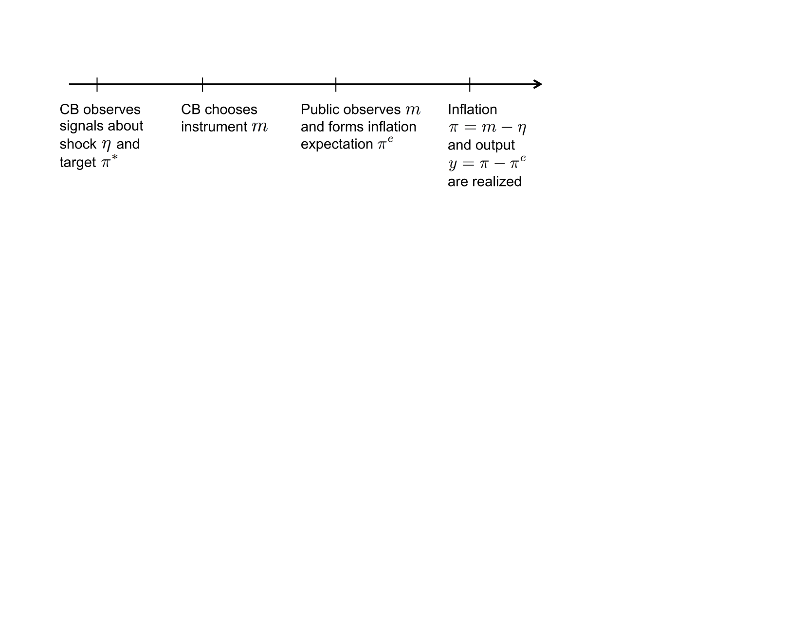
Since inflation $\pi$ is determined by the monetary instrument $m$ and the operational shock $\eta$, and the CB has a signal about $\eta$, the public makes inferences about $\pi$ (equivalently, $\eta$) from $m$. Consequently, the CB’s choice of $m$ has both a direct effect on its payoff by affecting inflation (and hence also output) and an indirect effect in how it affects the public’s inflation expectation. The latter is the signaling effect of monetary policy.

All aspects of the model except the realization of the CB’s private information, $s_{\eta }$ and $s_{{\pi }^{\ast }}$, are common knowledge. We will study pure strategy (Perfect) Bayesian equilibria, which for our purposes can be described entirely by the CB’s monetary policy strategy $m(s_{\eta },s_{{\pi }^{\ast }})$. For any on-the-equilibrium path $m$, the public’s inflation expectation, ${\pi }^e(m)\equiv 𝔼[\pi \mid m]$, is determined by Bayes rule. Off path beliefs will not play a material role in our analysis. Given any ${\pi }^e(m)$, we can substitute (1) and (2) into (3) and rewrite the CB’s objective as choosing $m$ to maximize

$$-𝔼[\underset{\text{output gap cost}}{\underbrace{\upsilon {(m-\eta -{\pi }^e(m)-y^{\ast })}^2}}+\underset{\text{excess inflation cost}}{\underbrace{{(m-\eta -{\pi }^{\ast })}^2}}\mid s_{\eta },s_{{\pi }^{\ast }}].$$ (4)

A key distinction between the operational shock $\eta$ and the inflation target ${\pi }^{\ast }$ is that given any policy choice $m$, inflation $\pi$ is only affected by $\eta$. Hence, the inflation expectation ${\pi }^e$ depends on the public’s beliefs about $\eta$ but not about ${\pi }^{\ast }$. Naturally, the CB’s choice of $m$ will depend on its beliefs about both $\eta$ and ${\pi }^{\ast }$.

We define welfare as the CB’s ex-ante expected utility from (3). Using the fact that $𝔼[y]=0$, we can use a standard mean-variance decomposition to express welfare as

$$\mathrm{Welfare}=-\underset{\begin{array}{c}\text{output volatility}\\ \text{cost}\end{array}}{\underbrace{\upsilon \mathrm{Var}[y]}}-\underset{\begin{array}{c}\text{excess inflation}\\ \text{volatility cost}\end{array}}{\underbrace{\mathrm{Var}[\pi -{\pi }^{\ast }]}}-\underset{\begin{array}{c}\text{avg. excess}\\ \text{inflation cost}\end{array}}{\underbrace{{\left(𝔼[\pi -{\pi }^{\ast }]\right)}^2}}.$$ (5)

It bears emphasis that interpreting this object as social welfare presumes that shocks to the CB’s policy objective, i.e., to the inflation target ${\pi }^{\ast }$, reflect socially optimal tradeoffs between output and inflation. In other words, we take both the operational shock $\eta$ and the inflation target ${\pi }^{\ast }$ as ultimately reflecting economic conditions. This perspective also justifies why the CB may not know ${\pi }^{\ast }$ precisely—${\pi }^{\ast }$ is the socially optimal level of inflation given underlying conditions, which the CB can estimate using the signal $s_{{\pi }^{\ast }}$.

2.2 Benchmarks

Our model has two pieces of private information for the CB: $s_{\eta }$ and $s_{{\pi }^{\ast }}$. We begin by showing what would happen if either of these variables were made common knowledge.

Proposition 1.

The following benchmarks hold:

1. Assume the signal of the operational shock, $s_{\eta }$, is common knowledge. There is a unique equilibrium; the CB chooses $m(\cdot )=\overline{\eta }+{\overline{\pi }}^{\ast }$, with $\overline{\eta }$ and ${\overline{\pi }}^{\ast }$ its expectations of the operational shock and the inflation target, and the public’s inflation expectation is ${\pi }^e(\cdot )=m-\overline{\eta }$. For any $\eta$, ${\pi }^{\ast }$, $s_{\eta }$, and $s_{{\pi }^{\ast }}$, output is $\overline{\eta }-\eta$ and excess inflation is $\overline{\eta }-\eta +{\overline{\pi }}^{\ast }-{\pi }^{\ast }$. Average excess inflation is $0$ and welfare is $-(1+\upsilon )𝔼[\mathrm{Var}[\eta |s_{\eta }]]-𝔼[\mathrm{Var}[{\pi }^{\ast }|s_{{\pi }^{\ast }}]]$.

2. Assume the signal of the inflation target, $s_{{\pi }^{\ast }}$, is common knowledge but the public does not know the CB’s signal $s_{\eta }$. There is an equilibrium that separates on $\overline{\eta }$: the CB chooses $m(\cdot )=\overline{\eta }+{\overline{\pi }}^{\ast }+\upsilon y^{\ast }$ and the public’s inflation expectation is ${\pi }^e(\cdot )={\overline{\pi }}^{\ast }+\upsilon y^{\ast }$, independent of $m$. In this equilibrium, for any $\eta$, ${\pi }^{\ast }$, $s_{\eta }$, and $s_{{\pi }^{\ast }}$, output is $\overline{\eta }-\eta$ and excess inflation is $\overline{\eta }-\eta +{\overline{\pi }}^{\ast }-{\pi }^{\ast }+\upsilon y^{\ast }$; average excess inflation is $\upsilon y^{\ast }$ and welfare is $-(1+\upsilon )𝔼[\mathrm{Var}[\eta |s_{\eta }]]-𝔼[\mathrm{Var}[{\pi }^{\ast }|s_{{\pi }^{\ast }}]]-{(\upsilon y^{\ast })}^2$.

(All proofs are in Appendix A.)

Part 1 of Proposition 1 says that if the CB could not fool the public about inflation (because the public sees the CB’s signal of the operational shock $s_{\eta }$ and it observes the monetary instrument $m$), and hence could not affect output, it would choose monetary policy to equate expected inflation with its best estimate of the inflation target. There is no average excess inflation, and welfare attains the maximum feasible level given the CB’s information constraints, i.e., given that it only observes signals of the operational shock and the inflation target.

Part 2 of Proposition 1 shows that when the CB has private information on the operational shock, its incentive to manipulate inflation expectations generates positive average excess inflation. The intuition is transparent: if the public thought the CB were playing the strategy from part 1, $m(\cdot )=\overline{\eta }+{\overline{\pi }}^{\ast }$, the CB could profitably deviate by raising $m$ slightly above the conjecture; such a deviation would produce an expected second-order cost from excess inflation, but yield a first-order output benefit through the surprise inflation. In equilibrium there is expected excess inflation of $\upsilon y^{\ast }$ conditional on any $s_{\eta }$ and $s_{{\pi }^{\ast }}$; inflation is, on average, above the CB’s preferred level given its information. The average excess inflation comes without any countervailing benefit, and welfare is lower than in part 1. In sum, the CB’s ability to manipulate inflation expectations is self-defeating.

Proposition 1 demonstrates an analog of the time-inconsistency or credibility problem going back to Kydland and Prescott (1977) and Barro and Gordon (1983b). If we had instead assumed that the public’s inflation expectation is formed prior to observing the monetary policy $m$—as in Barro and Gordon (1983a, b)—then there would be excess inflation even if the public knew the CB’s signal about the operational shock, contrary to part 1 of Proposition 1. We make our timing assumption because, as already discussed in the introduction, there is evidence that monetary policy has a signaling role and affects public expectations, and we wish to focus on this aspect of the problem. It is not important for our message that all firms/consumers be able to adjust their expectations (and/or their behavior) in response to monetary policy; only that some do.

A direct implication of Proposition 1 is that if the CB only has one piece of private information, a more informed or competent CB leads to higher welfare. Formally:

Corollary 1.

If either of the two signals $s_{\eta }$ or $s_{{\pi }^{\ast }}$ is common knowledge, welfare is increasing in the variances of the CB’s posterior means, $\mathrm{Var}[\overline{\eta }]$ and $\mathrm{Var}[{\overline{\pi }}^{\ast }]$.

2.3 Assumptions on the information structure

In the remainder of the paper we study the setting in which the signals about both the operational shock and the inflation target, $s_{\eta }$ and $s_{{\pi }^{\ast }}$ respectively, are the CB’s private information. For tractability, we will assume hereafter a normal-normal information structure. Using the notation $𝒩(\mu ,{\sigma }^2)$ to denote a normal distribution with mean $\mu$ and variance ${\sigma }^2$ or, equivalently, precision $1/{\sigma }^2$, we maintain:

Assumption 1.

The variables $\eta$, ${\pi }^{\ast }$, ${\epsilon }_{\eta }$, and ${\epsilon }_{{\pi }^{\ast }}$ are all independent normal, with $x\sim 𝒩({\mu }_x,{\sigma }_x^2)$ and ${\epsilon }_x\sim 𝒩(0,1/{\tau }_x)$ for $x\in \{\eta ,{\pi }^{\ast }\}$.

A notational point bears emphasis: for $x\in \{\eta ,{\pi }^{\ast }\}$, ${\tau }_x\ne 1/{\sigma }_x^2$, i.e., ${\tau }_x$ is not the precision of $x$; it is instead the precision of $s_x$, the signal about $x$. Also, with some abuse of notation, we allow for ${\tau }_x=\mathrm{\infty }$, which corresponds to the CB being fully informed about $x$.

It is a standard result that for each $x\in \{\eta ,{\pi }^{\ast }\}$, the CB’s expectation of $x$ after observing the signal $s_x=x+{\epsilon }_x$ is given by

$\overline{x}(s_x)$ $={\displaystyle \frac{{\mu }_x/{\sigma }_x^2+{\tau }_x{s}_x}{1/{\sigma }_x^2+{\tau }_x}}.$ (6)

The variance of this posterior mean over all signal realizations is

$\mathrm{Var}[\overline{x}]$ $={\displaystyle \frac{{\sigma }_x^4}{{\sigma }_x^2+1/{\tau }_x}}.$ (7)

The variance $\mathrm{Var}[\overline{x}]$ is in the range $(0,{\sigma }_x^2]$ and is increasing in the signal precision ${\tau }_x$; a more competent CB is one with larger ${\tau }_x$ and, for any given ${\sigma }_x^2$, a larger $\mathrm{Var}[\overline{x}]$. Moreover, for any realization $s_x$, the conditional distribution of $x$ is given by $x\mid s_x\sim 𝒩(\overline{x}(s_x),{\sigma }_x^2-\mathrm{Var}[\overline{x}])$.

As is common with normal distributions and quadratic objectives, we study linear equilibria in which the public’s expectations of the operational shock ${\eta }^e\equiv 𝔼[\eta \mid m]$ and of the inflation target ${\pi }^e\equiv 𝔼[\pi \mid m]$ are given by

${\eta }^e(m)$ $=Lm+K,$ (8)

${\pi }^e(m)$ $=m-{\eta }^e(m)=(1-L)m-K,$ (9)

for some constants $L$ and $K$.

3 Competence Can Reduce Credibility

To illustrate our main point transparently about why limiting the CB’s information about the operational shock, $\eta$, can be beneficial, consider a simplified version of our model in which the CB’s output objective is linearized. (We turn to the general analysis in Section 4.) Specifically, simplify the CB’s payoff to be

$$2\gamma y-{(\pi -{\pi }^{\ast })}^2,$$ (10)

where $\gamma >0$ is a commonly-known constant. In this specification, the marginal benefit of output is $2\gamma$ no matter the output $y$. In our main model in which the CB’s payoff is given by (3), the marginal benefit of output at $y=0$ is $2\upsilon y^{\ast }$. Hence, when $y^{\ast }>0$ and $\gamma =\upsilon y^{\ast }$, the linear output objective in (10) is a first-order approximation about $y=0$ to the quadratic output objective in (3). The approximation becomes perfect for fixed $\gamma >0$ (in the sense that for any given $y$, the marginal benefit of output tends to $2\gamma$) as we take $y^{\ast }\to \mathrm{\infty }$ and $\upsilon \to 0$ in (3) while maintaining $\upsilon y^{\ast }=\gamma$. A simplification afforded by linearizing the output objective is that, because $2\gamma 𝔼[y]=0$, welfare depends only on the ex-ante mean and variance of excess inflation. We can therefore rewrite welfare from (5) as

$$\mathrm{Welfare}=-\underset{\begin{array}{c}\text{excess inflation}\\ \text{volatility cost}\end{array}}{\underbrace{\mathrm{Var}[\pi -{\pi }^{\ast }]}}-\underset{\begin{array}{c}\text{avg. excess}\\ \text{inflation cost}\end{array}}{\underbrace{{\left(𝔼[\pi -{\pi }^{\ast }]\right)}^2}}.$$

Given linear public expectations of the form (8) and (9), it is routine (see the proof of Proposition 2) that the CB’s optimal choice of monetary instrument $m$ is given by

$m(s_{\eta },s_{\pi }^{\ast })=\overline{\eta }(s_{\eta })+{\overline{\pi }}^{\ast }(s_{{\pi }^{\ast }})+\gamma L.$ (11)

In turn, given a CB strategy of the form (11), standard results about updating with normal information (DeGroot, 1970) imply that the public’s expectations ${\eta }^e(m)$ and ${\pi }^e(m)$ take a linear form; see Lemma A.1 in Appendix A. An equilibrium is found by matching coefficients to solve for the constants $L$ and $K$.

Proposition 2.

Consider the linearized CB’s objective (10). There is a unique linear equilibrium: the CB’s plays (11) and the public’s expectations are (8) and (9), with

$L$ $={\displaystyle \frac{\mathrm{Var}[\overline{\eta }]}{\mathrm{Var}[\overline{\eta }]+\mathrm{Var}[{\overline{\pi }}^{\ast }]}}.$ (12)

Average excess inflation is $\gamma L$, the variance of excess inflation is $\left({\sigma }_{\eta }^2-\mathrm{Var}[\overline{\eta }]\right)-\left({\sigma }_{{\pi }^{\ast }}^2-\mathrm{Var}[{\overline{\pi }}^{\ast }]\right)$, and

$$\mathrm{Welfare}=-\left({\sigma }_{\eta }^2-\mathrm{Var}[\overline{\eta }]\right)-\left({\sigma }_{{\pi }^{\ast }}^2-\mathrm{Var}[{\overline{\pi }}^{\ast }]\right)-{(\gamma L)}^2.$$ (13)

To understand Proposition 2, observe that if the public knew $s_{{\pi }^{\ast }}$ but not $s_{\eta }$, there would be a separating equilibrium in which the public’s inflation expectation ${\pi }^e$ is independent of the instrument $m$, just as in Proposition 1 part 2. This would induce a temptation for the CB to increase $m$ (and hence expected inflation and expected output) until, in expectation, the constant marginal benefit of extra output were equalized with the increasing marginal cost of excess inflation. This would result in average excess inflation of $𝔼[\pi -{\pi }^{\ast }]=\gamma$, and society would bear the cost of this average excess inflation without any output benefit; welfare would be $-\left({\sigma }_{\eta }^2-\mathrm{Var}[\overline{\eta }]\right)-\left({\sigma }_{{\pi }^{\ast }}^2-\mathrm{Var}[{\overline{\pi }}^{\ast }]\right)-{\gamma }^2$.

By contrast, when there is uncertainty about $s_{{\pi }^{\ast }}$ as well, the public’s inflation expectation increases with the CB’s instrument. Specifically, ${\pi }^e(m)=(1-L)m-K$, and therefore, using Equation 12, $\frac{\mathrm{d}{\pi }^e(m)}{\mathrm{d}m}=1-L=\mathrm{Var}[{\overline{\pi }}^{\ast }]/\left(\mathrm{Var}[\overline{\eta }]+\mathrm{Var}[{\overline{\pi }}^{\ast }]\right)$. Increasing the instrument $m$ thus becomes less attractive to the CB: there is a smaller expected marginal output benefit for the same expected increase in inflation. Or, to put it differently, achieving the same expected marginal output benefit by fooling the public would require bearing a higher expected cost of inflation. So while the CB still cannot increase average output in equilibrium, the commitment problem becomes less severe and average inflation goes down. Average excess inflation becomes $𝔼[\pi -{\pi }^{\ast }]={\sigma }_{\eta }^2/\left(\mathrm{Var}[\overline{\eta }]+\mathrm{Var}[{\overline{\pi }}^{\ast }]\right)\gamma ,$ which is lower than $\gamma$, the average excess inflation when $s_{{\pi }^{\ast }}$ is commonly known. This decrease in average excess inflation gives a corresponding increase in welfare of ${((1-L)\gamma )}^2={\gamma }^2{\left(\mathrm{Var}[{\overline{\pi }}^{\ast }]/\left(\mathrm{Var}[\overline{\eta }]+\mathrm{Var}[{\overline{\pi }}^{\ast }]\right)\right)}^2$.

Consequently, there is a social benefit when the equilibrium value of $L$ is lower, i.e., when the public’s inflation expectation is more sensitive to the CB’s choice of instrument $m$; as just explained, this mitigates the CB’s commitment problem. Equation 12 tells us that greater sensitivity of inflation expectation can be achieved by either increasing $\mathrm{Var}[{\overline{\pi }}^{\ast }]$ or decreasing $\mathrm{Var}[\overline{\eta }]$; equivalently, by increasing the precision of the CB’s information about the inflation target, ${\tau }_{{\pi }^{\ast }}$, or decreasing that about the operational shock, ${\tau }_{\eta }$. In either case, the public attributes changes in $m$ more so to changes in the CB’s (estimated) inflation target and less so to the CB simply offsetting (estimated) economic shocks. Of course, changes in the CB’s competence also have direct effects on welfare, because they affect the CB’s ability to tailor inflation $\pi$ to the target ${\pi }^{\ast }$. As is intuitive and confirmed by expression (13), the direct effect always favors the CB being better informed.

Corollary 2.

Consider the linearized CB’s objective (10). Welfare is higher when the CB is more informed about the inflation target ${\pi }^{\ast }$, i.e., when its precision ${\tau }_{{\pi }^{\ast }}$ is higher. Welfare can increase or decrease when the CB is more informed about the operational shock $\eta$, i.e., when its precision ${\tau }_{\eta }$ is higher.

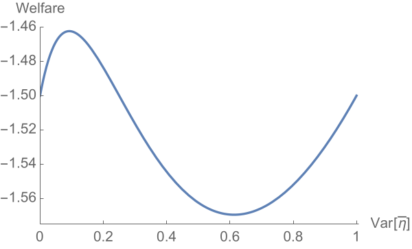
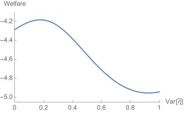
As seen in Figure 2, the optimal level of information about the operational shock can be interior, i.e., the optimal precision ${\tau }_{\eta }$ can be finite, even though welfare need not be single-peaked in the precision.

Figure 2: Higher precision of the CB’s observation of the operational shock $\eta$ has ambiguous welfare effects. (Increasing precision ${\tau }_{\eta }$ from $0$ to $\mathrm{\infty }$ corresponds to increasing $\mathrm{Var}[\overline{\eta }]$ from 0 to 1.) Parameters are ${\sigma }_{\eta }^2=1$, $\gamma =2.5$, ${\sigma }_{{\pi }^{\ast }}^2=2$, and ${\tau }_{{\pi }^{\ast }}=1$.

4 General Analysis

4.1 Solving the model

Armed with the intuitions from linearization, we now solve the model. When the public holds the linear conjecture of Equation 8 and Equation 9, the first-order condition for the CB’s choice of instrument $m$—plugging expected inflation ${\pi }^e=(1-L)m-K$ into the objective (4)—yields

$$-2\upsilon L(Lm-\overline{\eta }(s_{\eta })+K-y^{\ast })-2(m-\overline{\eta }(s_{\eta })-{\overline{\pi }}^{\ast }(s_{{\pi }^{\ast }}))=0.$$

As the CB’s problem is concave, solving for $m$ gives the CB’s optimal choice of

$m(s_{\eta },s_{{\pi }^{\ast }})$ $=\overline{\eta }(s_{\eta }){\displaystyle \frac{1+\upsilon L}{1+\upsilon L^2}}+{\overline{\pi }}^{\ast }(s_{{\pi }^{\ast }}){\displaystyle \frac{1}{1+\upsilon L^2}}+{\displaystyle \frac{\upsilon L(y^{\ast }-K)}{1+\upsilon L^2}}.$ (14)

Lemma 1.

Suppose the CB uses the strategy in Equation 14. Then, conditional on instrument $m$, the public’s posterior belief about the operational shock $\eta$ has mean ${\mu }_{\eta |m}$ given by

${\mu }_{\eta \mid m}$ $={\displaystyle \frac{(1+\upsilon L)(1+\upsilon L^2)\mathrm{Var}[\overline{\eta }]}{{(1+\upsilon L)}^2\mathrm{Var}[\overline{\eta }]+\mathrm{Var}[{\overline{\pi }}^{\ast }]}}m$

$+{\mu }_{\eta }-{\displaystyle \frac{(1+\upsilon L)\mathrm{Var}[\overline{\eta }]}{{(1+\upsilon L)}^2\mathrm{Var}[\overline{\eta }]+\mathrm{Var}[{\overline{\pi }}^{\ast }]}}\left({\mu }_{\eta }(1+\upsilon L)+{\mu }_{{\pi }^{\ast }}+\upsilon L(y^{\ast }-K)\right).$

Matching coefficients from the conjectured beliefs ${\eta }^e(m)=Lm+K$ to the corresponding formula in Lemma 1, in a linear equilibrium $L$ must satisfy

$L={\displaystyle \frac{(1+\upsilon L)\left(1+\upsilon L^2\right)\mathrm{Var}[\overline{\eta }]}{{(1+\upsilon L)}^2\mathrm{Var}[\overline{\eta }]+\mathrm{Var}[{\overline{\pi }}^{\ast }]}}.$ (15)

There are two solutions, only one of which is positive:

$L$ $={\displaystyle \frac{\upsilon -1-\mathrm{Var}[{\overline{\pi }}^{\ast }]/\mathrm{Var}[\overline{\eta }]+\sqrt{4\upsilon +{\left(\upsilon -1-\mathrm{Var}[{\overline{\pi }}^{\ast }]/\mathrm{Var}[\overline{\eta }]\right)}^2}}{2\upsilon }}\in (0,1).$ (16)

We focus on increasing equilibria (i.e., those in which both ${\eta }^e(m)$ and ${\pi }^e(m)$ are nondecreasing), and hence the above solution.

Lemma 2.

The equilibrium sensitivity constant $L$ defined by Equation 16 has the following properties:

1. , with $\underset{\mathrm{Var}[{\overline{\pi }}^{\ast }]\to 0}{lim}L=1$ and $\underset{\mathrm{Var}[{\overline{\pi }}^{\ast }]\to \mathrm{\infty }}{lim}L=0$;

2. $\frac{\partial L}{\partial \mathrm{Var}[\overline{\eta }]}>0$, with $\underset{\mathrm{Var}[\overline{\eta }]\to 0}{lim}L=0$ and $\underset{\mathrm{Var}[\overline{\eta }]\to \mathrm{\infty }}{lim}L=1$;

3. $\frac{\partial L}{\partial \upsilon }>0$, with $\underset{\upsilon \to 0}{lim}L=\frac{\mathrm{Var}[\overline{\eta }]}{\mathrm{Var}[\overline{\eta }]+\mathrm{Var}[{\overline{\pi }}^{\ast }]}$ and $\underset{\upsilon \to \mathrm{\infty }}{lim}L=1$.

The first two parts of the Lemma imply that, as before, the sensitivity of the public’s inflation expectation to the CB’s action, which is measured by $1-L$, is higher when the CB is more informed about the inflation target ${\pi }^{\ast }$ or less informed about the operational shock $\eta$. Part 3 of Lemma 2 confirms that the limit of $L$ as $v\to 0$ is $\frac{\mathrm{Var}[\overline{\eta }]}{\mathrm{Var}[\overline{\eta }]+\mathrm{Var}[{\overline{\pi }}^{\ast }]}$, the formula for $L$ from (12) under the linearized objective (10). Recall that the linearized objective is the limit of the objective (3) as we jointly take $y^{\ast }\to \mathrm{\infty }$ and $\upsilon \to 0$, noting that $y^{\ast }$ does not appear in the expression for $L$.

One can again match coefficients from Lemma 1 to those in (8) to solve for the constant $K$ in the equilibrium beliefs and strategy functions. Here it is convenient to first plug in the equilibrium relationship from (15) of $\frac{(1+\upsilon L)\mathrm{Var}[\overline{\eta }]}{{(1+\upsilon L)}^2\mathrm{Var}[\overline{\eta }]+\mathrm{Var}[{\overline{\pi }}^{\ast }]}=\frac{L}{1+\upsilon L^2}$ into the expression in Lemma 1, which yields

$$K=-\upsilon L^2{y}^{\ast }+{\mu }_{\eta }(1-L)-{\mu }_{{\pi }^{\ast }}L.$$ (17)

Proposition 3.

There is a unique increasing linear equilibrium; the public has beliefs ${\eta }^e(m)=Lm+K$ and ${\pi }^e(m)=(1-L)m-K$, and the CB plays (14), with $L$ and $K$ given by Equation 16 and Equation 17. In this equilibrium, variance of output, variance of inflation, expected excess inflation, and welfare are respectively given by:

$\mathrm{Var}[y]$ $=({\sigma }_{\eta }^2-\mathrm{Var}[\overline{\eta }])+{\left({\displaystyle \frac{1-L}{1+\upsilon L^2}}\right)}^2\mathrm{Var}[\overline{\eta }]+{\left({\displaystyle \frac{L}{1+\upsilon L^2}}\right)}^2\mathrm{Var}[{\overline{\pi }}^{\ast }],$

$\mathrm{Var}[\pi -{\pi }^{\ast }]$ $=({\sigma }_{\eta }^2-\mathrm{Var}[\overline{\eta }])+{\left({\displaystyle \frac{\upsilon L(1-L)}{1+\upsilon L^2}}\right)}^2\mathrm{Var}[\overline{\eta }]+({\sigma }_{{\pi }^{\ast }}^2-\mathrm{Var}[{\overline{\pi }}^{\ast }])+{\left({\displaystyle \frac{\upsilon L^2}{1+\upsilon L^2}}\right)}^2\mathrm{Var}[{\overline{\pi }}^{\ast }],$

$𝔼[\pi -{\pi }^{\ast }]$ $=\upsilon L{y}^{\ast },$

$\mathrm{Welfare}$ $=-\upsilon (1-L)\mathrm{Var}[\overline{\eta }]-(\upsilon +1)({\sigma }_{\eta }^2-\mathrm{Var}[\overline{\eta }])-({\sigma }_{{\pi }^{\ast }}^2-\mathrm{Var}[{\overline{\pi }}^{\ast }])-{\upsilon }^2{L}^2{(y^{\ast })}^2.$ (18)

As detailed in the Proposition’s proof, the welfare expression (18) is obtained by substituting the expressions for output variance, inflation variance, and expected excess inflation into (5), and then simplifying using (15). This welfare expression turns out to be convenient for our comparative statics.

4.2 More information about the inflation target

As in Section 3, better CB information about the inflation target ${\pi }^{\ast }$ is always desirable:

Proposition 4.

Welfare increases in ${\tau }_{{\pi }^{\ast }}$, the precision of the CB’s information about the inflation target ${\pi }^{\ast }$.

The proof consists of establishing that the welfare expression (18) increases with $\mathrm{Var}[{\overline{\pi }}^{\ast }]$, the variance the CB’s posterior mean about the inflation target ${\pi }^{\ast }$.

4.3 More information about the operational shock

To determine how welfare varies with information about the operational shock $\eta$, it will be convenient to rewrite the welfare expression stripped of terms that do not depend on $\mathrm{Var}[\overline{\eta }]$ (nor on $L$, which itself depends on $\mathrm{Var}[\overline{\eta }]$). Removing these terms from (18), define

$W(\mathrm{Var}[\overline{\eta }])\equiv (\upsilon L+1)\mathrm{Var}[\overline{\eta }]-{\upsilon }^2{L}^2{(y^{\ast })}^2,$ (19)

where $L$ depends on $\upsilon$, $\mathrm{Var}[\overline{\eta }]$, and $\mathrm{Var}[{\overline{\pi }}^{\ast }]$ as given by (16). At any given set of parameters, the welfare impact of improving information about the operational shock, i.e., increasing $\mathrm{Var}[\overline{\eta }]$, is quantitatively identical to the impact on $W$. We denote the derivative of $W$ by $W^{\prime }$.

The function $W$ depends on $y^{\ast }$, $\upsilon$, and $\mathrm{Var}[{\overline{\pi }}^{\ast }]$, but is independent of the ex-ante variances ${\sigma }_{{\pi }^{\ast }}^2$ and ${\sigma }_{\eta }^2$. However, ${\sigma }_{\eta }^2$ determines the relevant domain of $\mathrm{Var}[\overline{\eta }]$. As the CB moves from no information about $\eta$ (${\tau }_{\eta }\to 0$) to full information $({\tau }_{\eta }=\mathrm{\infty })$, the value $\mathrm{Var}[\overline{\eta }]$ covers the interval $(0,{\sigma }_{\eta }^2]$. So to explore the effect of information about $\eta$ on welfare, it will be useful to first characterize $W(\mathrm{Var}[\overline{\eta }])$ on the unrestricted domain $\mathrm{Var}[\overline{\eta }]\in (0,\mathrm{\infty })$. Then, given ${\sigma }_{\eta }^2$, we truncate the domain to $(0,{\sigma }_{\eta }^2]$ to analyze the welfare effect of information about $\eta$.

First consider the behavior of $W$ at the limits of the domain $\mathrm{Var}[\overline{\eta }]\in (0,\mathrm{\infty })$.

Lemma 3.

The following limits hold:

1. As $\mathrm{Var}[\overline{\eta }]\to 0$, $W(\mathrm{Var}[\overline{\eta }])\to 0$ and $W^{\prime }(\mathrm{Var}[\overline{\eta }])\to 1$.

2. As $\mathrm{Var}[\overline{\eta }]\to \mathrm{\infty }$, $W(\mathrm{Var}[\overline{\eta }])\to \mathrm{\infty }$ and $W^{\prime }(\mathrm{Var}[\overline{\eta }])\to \upsilon +1$.

In part 1 of Lemma 3, the limit $W(\mathrm{Var}[\overline{\eta }])\to 0$ as $\mathrm{Var}[\overline{\eta }]\to 0$ establishes a normalization that the transformed welfare $W$ goes to 0 as we approach no information about the operational shock $\eta$. The positive derivative as $\mathrm{Var}[\overline{\eta }]\to 0$ implies that:

Proposition 5.

Welfare increases in ${\tau }_{\eta }$, the precision of the CB’s information about the operational shock, in a neighborhood of ${\tau }_{\eta }=0$. Thus, it is never optimal for the CB to have no private information about the operational shock.

The implications of part 2 of Lemma 3 are more subtle because full information about the operational shock $\eta$ (${\tau }_{\eta }=\mathrm{\infty }$) corresponds to $\mathrm{Var}[\overline{\eta }]={\sigma }_{\eta }^2$ rather than $\mathrm{Var}[\overline{\eta }]\to \mathrm{\infty }$. So the positive derivative as $\mathrm{Var}[\overline{\eta }]\to \mathrm{\infty }$ does not say that better information about $\eta$ improves welfare if the CB already has close to full information; rather, it tells us that when ${\sigma }_{\eta }^2$ is sufficiently large, which corresponds to large ex-ante uncertainty about the operational shock $\eta$, better information about this shock improves welfare when the CB is already sufficiently well-informed about it.

It follows that for any given $\upsilon$, $y^{\ast }$, and $\mathrm{Var}[{\overline{\pi }}^{\ast }]$, there are two possibilities. First, $W$ can be increasing in $\mathrm{Var}[\overline{\eta }]$ over the entire domain $(0,\mathrm{\infty })$. In this case more information about the operational shock $\eta$ always improves welfare. Second, while $W$ is increasing at low and high $\mathrm{Var}[\overline{\eta }]$, it may be nonmonotonic over $(0,\mathrm{\infty })$. In this case the welfare effect of the CB’s information about $\eta$ depends on its variance ${\sigma }_{\eta }^2$. For ${\sigma }_{\eta }^2$ small, $W$ will be increasing on $(0,{\sigma }_{\eta }^2)$, and so welfare will be increasing in information about the operational shock. The welfare-maximizing value will be $\mathrm{Var}[\overline{\eta }]={\sigma }_{\eta }^2$, corresponding to full precision ${\tau }_{\eta }=\mathrm{\infty }$. For some intermediate values of ${\sigma }_{\eta }^2$, welfare will be increasing in $\mathrm{Var}[\overline{\eta }]$ on some regions and decreasing in others, and the welfare-maximizing value of $\mathrm{Var}[\overline{\eta }]$ (and hence of ${\tau }_{\eta }$) will be interior. Finally, for ${\sigma }_{\eta }^2$ sufficiently large, welfare will be increasing in $\mathrm{Var}[\overline{\eta }]$ on some regions and decreasing in others, but the welfare-maximizing value will be still be full information about the operational shock: $\mathrm{Var}[\overline{\eta }]={\sigma }_{\eta }^2$, or equivalently, ${\tau }_{\eta }=\mathrm{\infty }$.

We next examine how parameters determine the aforementioned (non)monotonicity. The two lemmas below consider how the shape of $W(\mathrm{Var}[\overline{\eta }])$ depends on the output target, $y^{\ast }$, and the weight the CB puts on the output gap, $\upsilon$. Recall that the sign of $W(\mathrm{Var}[\overline{\eta }])$ compares welfare to when the CB is uninformed about the operational shock $\eta$: means that welfare is lower than at the limit of no information (Lemma 3 part 2).

Lemma 4.

Fix any $\upsilon >0$ and $\mathrm{Var}[{\overline{\pi }}^{\ast }]>0$.

1. There exist cutoffs such that (i) if , then $W(\mathrm{Var}[\overline{\eta }])$ is increasing over $(0,\mathrm{\infty })$, and (ii) if $y^{\ast }>y_h^{\ast }$ then $W(\mathrm{Var}[\overline{\eta }])$ is nonmonotonic over $(0,\mathrm{\infty })$.

2. Fix $\mathrm{Var}[\overline{\eta }]>0$ as well. For $y^{\ast }$ sufficiently high,

Lemma 5.

Fix any $y^{\ast }>0$ and $\mathrm{Var}[{\overline{\pi }}^{\ast }]>0$.

1. There exist cutoffs such that (i) if , then $W(\mathrm{Var}[\overline{\eta }])$ is increasing over $(0,\mathrm{\infty })$, and (ii) if $\upsilon >{\upsilon }_h$ then $W$ is nonmonotonic over $(0,\mathrm{\infty })$.

2. Fix $\mathrm{Var}[\overline{\eta }]>0$ as well. For $\upsilon$ sufficiently high, .

A higher output target $y^{\ast }$ or (given $y^{\ast }>0$) a higher weight $\upsilon$ on output in the CB’s objective correspond to a more inflation-biased CB. Thus, a takeaway from Lemmas 3–5 is that more information about the operational shock $\eta$ is always desirable if and only if the CB is not too inflation biased. In other words, the tradeoff when increasing ${\tau }_{\eta }$—with direct benefit of make the CB better informed about the operational shock, but with strategic cost of hurting the CB’s credibility by lowering the public’s inflation-expectation sensitivity—turns on how inflation biased the CB is.

Proposition 6.

The CB’s inflation bias has the following welfare consequences for the CB’s information about the operational shock $\eta$:

1. (Low inflation bias.) If the output target $y^{\ast }$ or weight on output $\upsilon$ is sufficiently small, then more information about $\eta$ (i.e., higher precision ${\tau }_{\eta }$) increases welfare.

2. (High inflation bias.)

   1. If $y^{\ast }$ or $\upsilon$ is sufficiently large (with $y^{\ast }>0$), then so long as there is sufficient ex-ante uncertainty about $\eta$ (i.e., ${\sigma }_{\eta }^2$ is large enough), welfare is nonmonotonic in information about $\eta$.

   2. For any ${\sigma }_{\eta }^2$, if $y^{\ast }$ or $\upsilon$ is sufficiently large (with $y^{\ast }>0$), then no information about $\eta$ (i.e., ${\tau }_{\eta }\approx 0$) is better than full information (i.e, ${\tau }_{\eta }=\mathrm{\infty }$), and the optimal precision of information is interior.

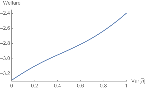
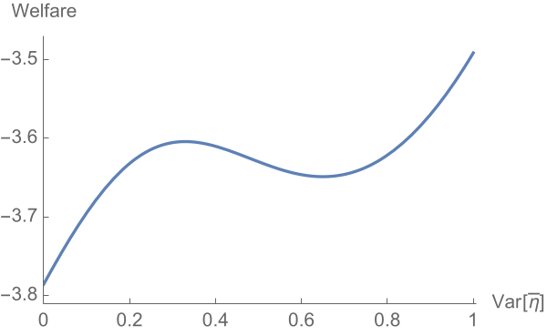
Figure 3 illustrates Proposition 6, showing how welfare depends on information about the operational shock $\eta$ for different levels of inflation bias. At low levels of inflation bias, more information about $\eta$ improves welfare. At higher levels, welfare is nonmonotonic in information about $\eta$ but is maximized at full information. At sufficiently high levels of inflation bias, no information improves on full information. While the figure shows different levels of inflation bias by fixing an output target $y^{\ast }>0$ and varying the weight $\upsilon$ the CB places on output, the qualitative results are identical when $\upsilon$ is fixed and $y^{\ast }$ varies.

(a) Low inflation bias: $\upsilon =1$.

(b) Medium inflation bias: $\upsilon =2$.

(c) High inflation bias: $\upsilon =3$.

Figure 3: Higher precision of the CB’s observation of the operational shock $\eta$ when the CB’s inflation bias is low, but can be harmful when the inflation bias is large. (Increasing precision ${\tau }_{\eta }$ from $0$ to $\mathrm{\infty }$ corresponds to increasing $\mathrm{Var}[\overline{\eta }]$ from 0 to 1.) Parameters are ${\sigma }_{\eta }^2=1$, ${\sigma }_{{\pi }^{\ast }}^2=2$, ${\tau }_{{\pi }^{\ast }}=3$, and $y^{\ast }=1$, with the values of $\upsilon$ indicated in each panel.

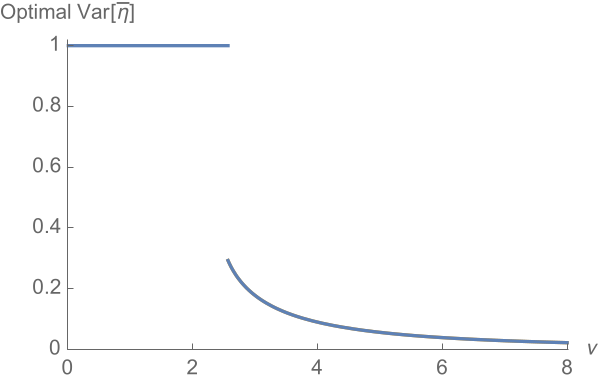
Consistent with Proposition 6, numerical analyses indicate that the optimal amount of information about the operational shock $\eta$ (i.e., the optimal precision ${\tau }_{\eta }$) is nonincreasing in the output target $y^{\ast }$ and the weight on output $\upsilon$; while this is straightforward to establish analytically for $y^{\ast }$, a proof for $\upsilon$ has been elusive. See Figure 4.

Figure 4: Numerically, higher inflation bias (here, higher weight $\upsilon$) reduces the welfare-maximizing competence $\mathrm{Var}[\overline{\eta }]$. ($\mathrm{Var}[\overline{\eta }]=1$ corresponds to full information about the operational shock $\eta$, i.e., precision ${\tau }_{\eta }=\mathrm{\infty }$, and $\mathrm{Var}[\overline{\eta }]\to 0$ corresponds to no information, i.e., ${\tau }_{\eta }\to 0$.) There is a discontinuity when the optimum switches from maximum competence to an interior solution. Parameters are ${\sigma }_{\eta }^2=1$, ${\sigma }_{{\pi }^{\ast }}^2=2$, ${\tau }_{{\pi }^{\ast }}=3$, and $y^{\ast }=1$.

We can also derive analogs of Lemmas 4 and 5 and Proposition 6 for different levels of $\mathrm{Var}[{\overline{\pi }}^{\ast }]$, the ex-ante variance of the CB’s belief about its inflation target. In a nutshell, low $\mathrm{Var}[{\overline{\pi }}^{\ast }]$ leads to nonmonotonicity of welfare in $\mathrm{Var}[\overline{\eta }]$, while high $\mathrm{Var}[{\overline{\pi }}^{\ast }]$ leads to monotonicity. Intuitively, when $\mathrm{Var}[{\overline{\pi }}^{\ast }]$ is high, the CB has significant private information about the inflation target and so the public’s inflation expectation is relatively sensitive to changes in monetary policy. In this case, the strategic gain conferred by a lower precision ${\tau }_{\eta }$ is always outweighed by the direct cost. Lemma B.1 and Proposition B.1 in Appendix B provide formal statements.

4.4 No private information about the inflation target

In Proposition 1 (part 2) and Corollary 1, we established that when the CB has no private information about the inflation target ${\pi }^{\ast }$, there is an equilibrium in which better information about the operational shock $\eta$ improves welfare. Here, we strengthen that point in the context of the equilibrium we have selected under the normal information structure.

Under the normal information structure, there are two ways in which the CB’s beliefs about ${\pi }^{\ast }$ can become common knowledge. First, the ex-ante uncertainty about ${\pi }^{\ast }$ may disappear: ${\sigma }_{{\pi }^{\ast }}^2\to 0$. Second, ${\pi }^{\ast }$ may be uncertain, but the CB’s signal about ${\pi }^{\ast }$ can become uninformative: the precision ${\tau }_{{\pi }^{\ast }}\to 0$. In either case, we will show that as we take the appropriate limit, the equilibrium of Proposition 3 has welfare increasing in the precision of information about the operational shock $\eta$.

When either ${\sigma }_{{\pi }^{\ast }}^2\to 0$ or ${\tau }_{{\pi }^{\ast }}\to 0$, it holds that $\mathrm{Var}[{\overline{\pi }}^{\ast }]\to 0$. As seen in Lemma 2, $\mathrm{Var}[{\overline{\pi }}^{\ast }]\to 0$ results in the equilibrium sensitivity constant $L\to 1$: the public infers that any increase or decrease in the CB’s monetary policy is due entirely to changes in the CB’s beliefs about the operational shock $\eta$. Proposition 3 shows that when $L\to 1$, the only effect of improved information about $\eta$ (i.e., higher $\mathrm{Var}[\overline{\eta }]$) is to reduce the variance of both output and excess inflation through the mechanical channel of reducing ${\sigma }_{\eta }^2-\mathrm{Var}[\overline{\eta }]$. Welfare goes up simply because the CB’s choice of monetary policy better matches $\eta$ when the signal about $\eta$ is less noisy.

Proposition 7.

Fix any $\delta >0$. As either the CB’s information about the inflation target becomes perfect (i.e., ${\tau }_{{\pi }^{\ast }}\to 0$) or the ex-ante uncertainty about the inflation target vanishes (i.e., ${\sigma }_{{\pi }^{\ast }}^2\to 0$), welfare is increasing in ${\tau }_{\eta }$, the precision of the CB’s information about the operational shock $\eta$, over the domain $(\delta ,\mathrm{\infty }]$.

To restate the point, any cost of increased central bank competence only emerges in our model when the CB has private information about the inflation target ${\pi }^{\ast }$.

5 Uncertainty over the output target

Having established our main results, we study in this section an alternative specification of the problem. We maintain that the CB seeks to maximize the expectation of (3), but now the inflation target ${\pi }^{\ast }$ is commonly known and the CB has private information about the other policy objective, the output target $y^{\ast }$. As in Moscarini (2007), maximizing (3) with an uncertain $y^{\ast }$ is equivalent to maximizing (3) with a commonly-known $y^{\ast }$ combined with CB private information about a shock to the output level. This shock could arise, for instance, from a TFP shock.

Our goal is to show that our paper’s main points go through in this alternative specification: in particular, the welfare effect of more CB information about the operational shock $\eta$ is ambiguous.

For tractability, as in Section 3, we will demonstrate this result under a simplified linearized version of (3). Objective (3) implies that the marginal benefit of output at $y=0$ (the expected output under rational expectations) is $2\upsilon y^{\ast }$. The first-order approximation of the quadratic objective (3) about $y=0$ is therefore (10) with $\gamma =\upsilon y^{\ast }$, as before. We hereafter work with the objective (10); welfare refers to the ex-ante expectation of (10). Unlike in Section 3 where there was uncertainty about ${\pi }^{\ast }$, that variable is now commonly known. Rather, uncertainty about $y^{\ast }$ in (3) translates into uncertainty about $\gamma$ in (10).

Assume the CB observes signals $s_{\eta }=\eta +{\epsilon }_{\eta }$ and, new to the current section, $s_{\gamma }=\gamma +{\epsilon }_{\gamma }$. The variables $\eta$, $\gamma$, ${\epsilon }_{\eta }$, and ${\epsilon }_{\gamma }$ are all independent normal, with $x\sim 𝒩({\mu }_x,{\sigma }_x^2)$ and ${\epsilon }_x\sim 𝒩(0,1/{\tau }_x)$ for $x\in \{\eta ,\gamma \}$. We maintain the earlier notation that $\overline{x}\equiv 𝔼[x|s_x]$ is the posterior mean of $x$ given signal $s_x$, and $\mathrm{Var}[\overline{x}]$ denotes the variance of this posterior mean over all signal realizations. Recall that $\mathrm{Var}[\overline{x}]\in (0,{\sigma }_x^2]$, and that for any fixed ${\sigma }_x^2$, a higher $\mathrm{Var}[\overline{x}]$ corresponds to a more precise signal $s_x$.

As before, we study increasing linear equilibria in which the public’s expectations ${\eta }^e\equiv 𝔼[\eta \mid m]$ and ${\pi }^e\equiv 𝔼[\pi \mid m]$ are given by (8) and (9), for some constants $L>0$ and $K$. Under these linear public expectations it is routine that the CB’s optimal choice of $m$ is given by

$$m(s_{\eta },s_{\gamma })=\overline{\eta }+\overline{\gamma }L+{\pi }^{\ast }.$$ (20)

The main result of this section is:

Proposition 8.

Consider output-target uncertainty instead of inflation-target uncertainty, with the linearized CB’s objective (10). There is a unique increasing linear equilibrium. The CB plays (20) and the public’s expectations are (8) and (9), with $L\in (0,1)$ given by

$L={\displaystyle \frac{2\sqrt{\mathrm{Var}[\overline{\eta }]}}{\sqrt{\mathrm{Var}[\overline{\eta }]}+\sqrt{\mathrm{Var}[\overline{\eta }]+4\mathrm{Var}[\overline{\gamma }]}}}.$ (21)

Average excess inflation is ${\mu }_{\gamma }L$, the variance of excess inflation is $\left({\sigma }_{\eta }^2-\mathrm{Var}[\overline{\eta }]\right)+L^2\mathrm{Var}[\overline{\gamma }]$, and

$\mathrm{Welfare}$ $=2𝔼[\gamma y]-\mathrm{Var}[\pi -{\pi }^{\ast }]-{\left(𝔼[\pi -{\pi }^{\ast }]\right)}^2$ (22)

$=L^2\mathrm{Var}[\overline{\gamma }]-\left({\sigma }_{\eta }^2-\mathrm{Var}[\overline{\eta }]\right)-L^2{\mu }_{\gamma }^2.$ (23)

Let us compare Proposition 8 with Proposition 2 of Section 3. The strategic effects of information here are entirely analogous to the specification in Section 3, with the output-benefit parameter $\gamma$ here taking the role of the inflation target ${\pi }^{\ast }$ there. The more information the CB has about $\gamma$, the more sensitive is the public’s inflation expectation to the CB’s action (a higher $\mathrm{Var}[\overline{\gamma }]$ leads to lower $L$). On the other hand, the more information the CB has about the operational shock $\eta$, the less sensitive is the public’s inflation expectation to the CB’s action (a higher $\mathrm{Var}[\overline{\eta }]$ leads to higher $L$). Both these points can be confirmed using Equation 21. Consequently, average excess inflation goes down in magnitude when the CB has more private information about $\gamma$ or less about $\eta$. This reduction of average excess inflation improves welfare, as seen from the third term on the right-hand side of (22).

Unlike in Section 3’s specification, however, there is now also an ex-ante cost to the CB from the public’s inflation expectation being more sensitive. The reason is that with a stochastic output-benefit parameter $\gamma$, the CB benefits ex-ante from an ability to tailor how much it surprises the public to the realization of $\gamma$. This is seen in the first term of (22): $𝔼[\gamma y]=L^2\mathrm{Var}[\overline{\gamma }]>0$ even though $𝔼[y]=0$. A more sensitive public’s inflation expectation (a lower $L$) makes it more costly for the CB to boost output even when doing so is particularly important.

We see from (23) that there is an overall welfare benefit from a more sensitive inflation expectation (a lower equilibrium $L$) when ${\mu }_{\gamma }>{\sigma }_{\gamma }$. In this case the CB aims to boost output by producing surprise inflation both on average (${\mu }_{\gamma }>0$) and with sufficiently high probability (${\mu }_{\gamma }>{\sigma }_{\gamma }\ge \sqrt{\mathrm{Var}[\overline{\gamma }]}$). Better information about the output-benefit parameter $\gamma$ then leads to higher welfare, since the only welfare effect is to reduce the equilibrium value of $L$. There is, however, a tradeoff from better information about the operational shock $\eta$: it reduces welfare through the strategic channel of increasing $L$, but it improves welfare through the direct channel of allowing the CB to better smooth inflation (captured by the $\mathrm{Var}[\overline{\eta }]$ term in (23)). The net welfare effect of increasing CB information about $\eta$ can go either way.

Summarizing these observations, the following corollary provides an analogous result to Corollary 2.

Corollary 3.

Consider output-target uncertainty instead of inflation-target uncertainty, with the linearized CB’s objective (10). If the CB seeks to produce surprise inflation both on average and with sufficiently high probability (i.e., ${\mu }_{\gamma }>{\sigma }_{\gamma }$), then welfare is higher when the CB is more informed about the output-benefit parameter $\gamma$ while welfare can increase or decrease when the CB is more informed about the operational shock $\eta$.

6 Conclusion

This paper has developed a signaling model of the central-bank credibility problem first pointed out by Kydland and Prescott (1977) and Barro and Gordon (1983a). A (benevolent) CB may benefit from increasing output through surprise inflation; the public anticipates the CB’s behavior, leading to excess inflation without any output benefit on average. The inefficiency owes to the CB’s private information about an operational shock that affects how monetary policy translates into inflation. Our main contribution is to analyze this interaction in the presence of public uncertainty about the CB’s policy objectives. When changes in the CB’s monetary policy must be attributed more to its private information about objectives than its private information about the operational shock, the public’s inflation expectation becomes more responsive to monetary policy. This increases the CB’s cost of producing surprise inflation and, in equilibrium, results in lower average inflation. Consequently, greater CB competence—in the sense of better information—about the operational shock comes at a strategic cost. When the CB is sufficiently inflation biased, less competence on this dimension can improve welfare.

There are, of course, other ways in which the CB’s signaling distortion can be mitigated. One avenue concerns transparency. Suppose that, prior to its policy choice, the CB can commit to provide the public with noisy signals of its information about the operational shock and its objectives. In light of the mechanism we have highlighted, it should be intuitive that there is a strategic benefit of making the signal about the operational shock more informative, as this would make the public’s inflation expectation more responsive to policy. Conversely, however, there is a strategic cost of making the signal about objectives more informative. Geraats (2007) and our own working paper, Frankel and Kartik (2015), explore these points in more detail.

Another avenue for transmitting private information is through strategic communication or “cheap talk” by the CB, as in Moscarini (2007) or Bassetto (2016). Indeed, our paper’s logic is related to that of Moscarini (2007), even though the mechanics are quite different. Moscarini studies a model in which the CB directly chooses inflation, $\pi$, contemporaneously with the public’s inflation-expectation formation; there is no signaling through this policy action. Instead, the CB can send a cheap-talk announcement about it’s single dimension of private information, which is the estimated inflation target ${\overline{\pi }}^{\ast }$ (using our notation). Cheap talk can be partially-informative because the CB benefits from lowering the public’s inflation expectation only up to a point: if the inflation expectation is too low relative to the CB’s estimated inflation target, then the CB must bear a cost of expected excess deflation () to avoid overshooting its output target. Intuitively, then, cheap talk will be more credible or informative when the public’s inflation expectation is more sensitive to the CB’s announcement. Moscarini shows that such increased sensitivity emerges when the CB is more competent—its inflation-target estimate is more accurate—because in that case the CB’s inflation choice places more weight on it’s inflation-target estimate relative to the public’s inflation expectation.

Thus, both Moscarini’s (2007) and our comparative statics are driven by the strategic effects of changes in CB competence on the public’s inflation-expectation sensitivity to the CB’s action: a policy action in our case, a cheap-talk announcement in his. Unlike our emphasis, however, Moscarini does not study channels by which greater competence can lower the inflation-expectation sensitivity. An interesting question is whether even in a cheap-talk framework, there are plausible dimensions of private information for which greater CB competence leads to lower inflation-expectation sensitivity and thereby reduces the credibility of communication.

Appendices

Appendix A Proofs

• Part 1: Since the public knows $s_{\eta }$ and $s_{{\pi }^{\ast }}$ is uninformative about $\eta$, it follows that for any choice of $m$, the public infers that ${\pi }^e=m-\overline{\eta }$. So, for any choice of $m$, realized output is $y=m-\eta -{\pi }^e=\overline{\eta }-\eta$. The CB’s objective (4) thus reduces to choosing $m$ to minimize the expected cost of excess inflation, $𝔼[{(m-\eta -{\pi }^{\ast })}^2\mid s_{\eta },s_{{\pi }^{\ast }}]$, which yields the solution $m=\overline{\eta }+{\overline{\pi }}^{\ast }$. The formulae for realized output and excess inflation follow from the CB’s strategy and the public’s inflation expectation. Substituting these into (5) yields welfare equal to $-(1+\upsilon )\mathrm{Var}[\overline{\eta }-\eta ]-\mathrm{Var}[{\overline{\pi }}^{\ast }-{\pi }^{\ast }]$, which simplifies to the expression in the proposition because for $x\in \{\eta ,{\pi }^{\ast }\}$,

  $$\mathrm{Var}[\overline{x}-x]=𝔼[\mathrm{Var}[\overline{x}-x|s_x]]+\mathrm{Var}[𝔼[\overline{x}-x|s_x]]=𝔼[\mathrm{Var}[\overline{x}-x|s_x]]=𝔼[\mathrm{Var}[x|s_x]].$$

  Part 2: If the CB uses the strategy $m(s_{\eta },s_{{\pi }^{\ast }})=\overline{\eta }+{\overline{\pi }}^{\ast }+\upsilon y^{\ast }$, then realized inflation is $\pi =m-\eta =\overline{\eta }-\eta +{\overline{\pi }}^{\ast }+\upsilon y^{\ast }$. Hence, the public’s expectation is ${\pi }^e=𝔼[\overline{\eta }-\eta +{\overline{\pi }}^{\ast }+\upsilon y^{\ast }]={\overline{\pi }}^{\ast }+\upsilon y^{\ast }$ for all $m$ (necessarily on the equilibrium path, and we extend to off-path $m$ as well). Given this belief, the CB’s objective (4) implies the program

  $$\underset{m}{\max }-𝔼\left[\upsilon {(m-\eta -{\overline{\pi }}^{\ast }-(1+\upsilon )y^{\ast })}^2+{(m-\eta -{\pi }^{\ast })}^2\mid s_{\eta },s_{{\pi }^{\ast }}\right].$$

  The objective is concave in $m$; the first-order condition

  $$2(1+\upsilon )(m-𝔼[\eta +{\pi }^{\ast }\mid s_{\eta },s_{{\pi }^{\ast }}]-\upsilon y^{\ast })=0$$

  solves for $m=\overline{\eta }+{\overline{\pi }}^{\ast }+\upsilon y^{\ast }$. The formulae for realized output and excess inflation follow straightforwardly from the CB’s strategy and the public’s inflation expectation, and welfare is derived analogously to part 1. ∎

• For $x\in \{\eta ,{\pi }^{\ast }\}$, the law of iterated variance implies $𝔼[\mathrm{Var}[x|s_x]]=\mathrm{Var}[x]-\mathrm{Var}[\overline{x}]$. The result follows from the welfare expressions in Proposition 1. ∎

Lemma A.1.

If the CB’s strategy is $m(s_{\eta },s_{{\pi }^{\ast }})=\overline{\eta }(s_{\eta })k_{\eta }+{\overline{\pi }}^{\ast }(s_{{\pi }^{\ast }})k_{{\pi }^{\ast }}+k_0$, then the public’s belief ${\eta }^e(m)$ is given by

${\eta }^e(m)=m{\displaystyle \frac{k_{\eta }\mathrm{Var}[\overline{\eta }]}{k_{\eta }^2\mathrm{Var}[\overline{\eta }]+k_{{\pi }^{\ast }}^2\mathrm{Var}[{\overline{\pi }}^{\ast }]}}+{\mu }_{\eta }-({\mu }_{\eta }{k}_{\eta }+{\mu }_{{\pi }^{\ast }}{k}_{{\pi }^{\ast }}+k_0){\displaystyle \frac{k_{\eta }\mathrm{Var}[\overline{\eta }]}{k_{\eta }^2\mathrm{Var}[\overline{\eta }]+k_{{\pi }^{\ast }}^2\mathrm{Var}[{\overline{\pi }}^{\ast }]}}.$

• From (6) and (7), the CB’s posterior mean of $\eta$ is $\overline{\eta }(s_{\eta })=\frac{\frac{{\mu }_{\eta }}{{\tau }_{\eta }}+s_{\eta }{\sigma }_{\eta }^2}{\frac{1}{{\tau }_{\eta }}+{\sigma }_{\eta }^2}$ with variance $\mathrm{Var}[\overline{\eta }]=({\sigma }_{\eta }^2+\frac{1}{{\tau }_{\eta }}){\left(\frac{{\sigma }_{\eta }^2}{\frac{1}{{\tau }_{\eta }}+{\sigma }_{\eta }^2}\right)}^2$. Likewise, the CB’s mean of ${\pi }^{\ast }$ is ${\overline{\pi }}^{\ast }(s_{{\pi }^{\ast }})=\frac{\frac{{\mu }_{{\pi }^{\ast }}}{{\tau }_{{\pi }^{\ast }}}+s_{{\pi }^{\ast }}{\sigma }_{{\pi }^{\ast }}^2}{\frac{1}{{\tau }_{{\pi }^{\ast }}}+{\sigma }_{{\pi }^{\ast }}^2}$ with variance $\mathrm{Var}[{\overline{\pi }}^{\ast }]=({\sigma }_{{\pi }^{\ast }}^2+\frac{1}{{\tau }_{{\pi }^{\ast }}}){\left(\frac{{\sigma }_{{\pi }^{\ast }}^2}{\frac{1}{{\tau }_{{\pi }^{\ast }}}+{\sigma }_{{\pi }^{\ast }}^2}\right)}^2$.

  These expressions let us calculate the joint distribution of $\eta$ and $m$ under the proposed linear strategy for $m$. Under this strategy, the two variables $\eta$ and $m$ are jointly normally distributed with the following distribution:

  One can now apply standard rules for conditional distributions of jointly normally distributed variables (e.g., DeGroot, 1970) to calculate the expectation of $\eta$ given $m$ as stated in the Lemma. ∎

• When the public’s expectations are (8) and (9), plugging (9) into (10) with the substitution $y=m-\eta -{\pi }^e(m)$ yields the maximization program:

  $$\underset{m}{\max }𝔼[2\gamma (Lm+K-\eta )-{(m-\eta -{\pi }^{\ast })}^2],$$

  which is concave in $m$. Solving the first-order condition proves optimality of the CB strategy (11). Lemma A.1 shows that when the CB plays (11), the public’s expectation of the economic shock $\eta$ is linear in $m$. Specifically, plugging $k_{\eta }=k_{{\pi }^{\ast }}=1$ into the Lemma, the coefficient on $m$ is equal to $\frac{\mathrm{Var}[\overline{\eta }]}{\mathrm{Var}[\overline{\eta }]+\mathrm{Var}[{\overline{\pi }}^{\ast }]}$. It follows that there is a unique linear equilibrium; the equilibrium has $L=\frac{\mathrm{Var}[\overline{\eta }]}{\mathrm{Var}[\overline{\eta }]+\mathrm{Var}[{\overline{\pi }}^{\ast }]}.$ The formulae for (average) excess inflation and welfare are then straightforward. ∎

• That welfare is increasing in ${\tau }_{{\pi }^{\ast }}$ follows from Proposition 2, specifically expressions (12) and (13), and from the fact that $\mathrm{Var}[{\overline{\pi }}^{\ast }]$ is increasing in ${\tau }_{{\pi }^{\ast }}$. Figure 2 demonstrates that increasing ${\tau }_{\eta }$ has an ambiguous effect on welfare. ∎

• The result follows from Lemma A.1 with $k_{\eta }=\frac{1+\nu L}{1+\nu L^2}$, $k_{{\pi }^{\ast }}=\frac{1}{1+\nu L^2}$, and $k_0=\frac{\nu L(y^{\ast }-K)}{1+\nu L^2}$. ∎

• Parts 1 and 2 are straightforward from differentiating and from evaluating limits. For part 3, both limits are straightforward applications of L’Hopital’s rule. To sign the derivative $\frac{\partial L}{\partial \upsilon }$, first differentiate to get

  $$\frac{\partial L}{\partial \upsilon }=\frac{1+\mathrm{Var}[{\overline{\pi }}^{\ast }]/\mathrm{Var}[\overline{\eta }]-\sqrt{{\left(\upsilon -1-\mathrm{Var}[{\overline{\pi }}^{\ast }]/\mathrm{Var}[\overline{\eta }]\right)}^2+4\upsilon }+\upsilon \frac{1-\mathrm{Var}[{\overline{\pi }}^{\ast }]/\mathrm{Var}[\overline{\eta }]+\upsilon }{\sqrt{{\left(\upsilon -1-\mathrm{Var}[{\overline{\pi }}^{\ast }]/\mathrm{Var}[\overline{\eta }]\right)}^2+4\upsilon }}}{2{\upsilon }^2}.$$

  Ignoring the positive denominator, multiplying the numerator by $\sqrt{{\left(\upsilon -1-\mathrm{Var}[{\overline{\pi }}^{\ast }]/\mathrm{Var}[\overline{\eta }]\right)}^2+4\upsilon }$, and simplifying yields

  $$\mathrm{sign}\frac{\partial L}{\partial \upsilon }=\mathrm{sign}\left(\left(1+\frac{\mathrm{Var}\left[{\overline{\pi }}^{\ast }\right]}{\mathrm{Var}\left[\overline{\eta }\right]}\right)\sqrt{{\left(\upsilon -1-\frac{\mathrm{Var}\left[{\overline{\pi }}^{\ast }\right]}{\mathrm{Var}\left[\overline{\eta }\right]}\right)}^2+4\upsilon }-\left(1+\frac{\mathrm{Var}\left[{\overline{\pi }}^{\ast }\right]}{\mathrm{Var}\left[\overline{\eta }\right]}\right)\left(1+\frac{\mathrm{Var}\left[{\overline{\pi }}^{\ast }\right]}{\mathrm{Var}\left[\overline{\eta }\right]}-\upsilon \right)-2\upsilon \right).$$

  It therefore suffices to show that

  $$\sqrt{{\left(\upsilon -1-\mathrm{Var}[{\overline{\pi }}^{\ast }]/\mathrm{Var}[\overline{\eta }]\right)}^2+4\upsilon }>\left(1+\mathrm{Var}[{\overline{\pi }}^{\ast }]/\mathrm{Var}[\overline{\eta }]-\upsilon \right)+\frac{2\upsilon }{1+\mathrm{Var}[{\overline{\pi }}^{\ast }]/\mathrm{Var}[\overline{\eta }]}.$$

  Squaring both sides, some simple algebra verifies that this inequality is true. ∎

• Observe that for $x\in \{\eta ,{\pi }^{\ast }\}$ it holds that $\mathrm{Cov}[x,\overline{x}(s_x)]=\mathrm{Var}[\overline{x}(s_x)]=\mathrm{Var}[\overline{x}]$ because $𝔼[x\mid \overline{x}]=\overline{x}$; we will use this fact below.

  To calculate $\mathrm{Var}[y]$, note that

  $$y=\pi -{\pi }^e=(m-\eta )-\left((1-L)m-K\right)=Lm-\eta +K.$$

  Substituting in $m$ from (14),

  $$y=\frac{L}{1+\upsilon L^2}\left(\overline{\eta }(s_{\eta })(1+\upsilon L)+{\overline{\pi }}^{\ast }(s_{{\pi }^{\ast }})+\upsilon L(y^{\ast }-K)\right)-\eta +K.$$

  Hence,

  $$\mathrm{Var}[y]={\left(\frac{L(1+\upsilon L)}{1+\upsilon L^2}\right)}^2\mathrm{Var}[\overline{\eta }]+{\left(\frac{L}{1+\upsilon L^2}\right)}^2\mathrm{Var}[{\overline{\pi }}^{\ast }]+{\sigma }_{\eta }^2-2\frac{L(1+\upsilon L)}{1+\upsilon L^2}\mathrm{Cov}[\overline{\eta }(s_{\eta }),\eta ].$$

  Substituting in $\mathrm{Cov}[\overline{\eta }(s_{\eta }),\eta ]=\mathrm{Var}[\overline{\eta }]$ and simplifying gives the desired expression.

Next, note that $\pi -{\pi }^{\ast }=m-\eta -{\pi }^{\ast }$. Substituting in $m$ from (14),

$$\pi -{\pi }^{\ast }=\frac{1+\upsilon L}{1+\upsilon L^2}\overline{\eta }(s_{\eta })+\frac{1}{1+\upsilon L^2}{\overline{\pi }}^{\ast }(s_{{\pi }^{\ast }})+\frac{\upsilon L(y^{\ast }-K)}{1+\upsilon L^2}-\eta -{\pi }^{\ast }.$$ (A.1)

Hence,

$\mathrm{Var}[\pi -{\pi }^{\ast }]=$ ${\left({\displaystyle \frac{1+\upsilon L}{1+\upsilon L^2}}\right)}^2\mathrm{Var}[\overline{\eta }]+{\left({\displaystyle \frac{1}{1+\upsilon L^2}}\right)}^2\mathrm{Var}[{\overline{\pi }}^{\ast }]+{\sigma }_{\eta }^2+{\sigma }_{{\pi }^{\ast }}^2$

$-2{\displaystyle \frac{1+\upsilon L}{1+\upsilon L^2}}\mathrm{Cov}[\overline{\eta }(s_{\eta }),\eta ]-2{\displaystyle \frac{1}{1+\upsilon L^2}}\mathrm{Cov}[{\overline{\pi }}^{\ast }(s_{{\pi }^{\ast }}),{\pi }^{\ast }].$

Substituting in $\mathrm{Cov}[\overline{\eta }(s_{\eta }),\eta ]=\mathrm{Var}[\overline{\eta }]$ and $\mathrm{Cov}[{\overline{\pi }}^{\ast }(s_{{\pi }^{\ast }}),{\pi }^{\ast }]=\mathrm{Var}[{\overline{\pi }}^{\ast }]$ and then simplifying gives the desired expression.

Equation A.1 implies

$𝔼[\pi -{\pi }^{\ast }]={\mu }_{\eta }\left({\displaystyle \frac{1+\upsilon L}{1+\upsilon L^2}}-1\right)+{\mu }_{{\pi }^{\ast }}\left({\displaystyle \frac{1}{1+\upsilon L^2}}-1\right)+{\displaystyle \frac{\upsilon L(y^{\ast }-K)}{1+\upsilon L^2}}.$ (A.2)

From Equation 17, it holds that

$$\frac{\upsilon L(y^{\ast }-K)}{1+\upsilon L^2}=\upsilon L{y}^{\ast }-{\mu }_{\eta }\left(\frac{1+\upsilon L}{1+\upsilon L^2}-1\right)-{\mu }_{{\pi }^{\ast }}\left(\frac{1}{1+\upsilon L^2}-1\right).$$

Substituting this expression back into Equation A.2 yields $𝔼[\pi -{\pi }^{\ast }]=\upsilon L{y}^{\ast }$.

It remains to derive the welfare expression (18). First, substituting in the above expressions for $\mathrm{Var}[y]$, $\mathrm{Var}[\pi -{\pi }^{\ast }]$, and $𝔼[\pi -{\pi }^{\ast }]$ into (5) yields

$\mathrm{Welfare}=$ $-{\left(\upsilon L{y}^{\ast }\right)}^2-v\left(({\sigma }_{\eta }^2-\mathrm{Var}[\overline{\eta }])+{\left({\displaystyle \frac{1-L}{1+\upsilon L^2}}\right)}^2\mathrm{Var}[\overline{\eta }]+{\left({\displaystyle \frac{L}{1+\upsilon L^2}}\right)}^2\mathrm{Var}[{\overline{\pi }}^{\ast }]\right)$

$-\left(({\sigma }_{\eta }^2-\mathrm{Var}[\overline{\eta }])+{\left({\displaystyle \frac{\upsilon L(1-L)}{1+\upsilon L^2}}\right)}^2\mathrm{Var}[\overline{\eta }]+({\sigma }_{{\pi }^{\ast }}^2-\mathrm{Var}[{\overline{\pi }}^{\ast }])+{\left({\displaystyle \frac{\upsilon L^2}{1+\upsilon L^2}}\right)}^2\mathrm{Var}[{\overline{\pi }}^{\ast }]\right).$

Simplifying yields

$\mathrm{Welfare}$ $=-{\displaystyle \frac{\upsilon {(1-L)}^2}{1+\upsilon L^2}}\mathrm{Var}[\overline{\eta }]-{\displaystyle \frac{\upsilon L^2}{1+\upsilon L^2}}\mathrm{Var}[{\overline{\pi }}^{\ast }]$

$-(v+1)({\sigma }_{\eta }^2-\mathrm{Var}[\overline{\eta }])-({\sigma }_{{\pi }^{\ast }}^2-\mathrm{Var}[{\overline{\pi }}^{\ast }])-{\upsilon }^2{L}^2{(y^{\ast })}^2.$ (A.3)

Equation 15 can be manipulated to get $\mathrm{Var}[{\overline{\pi }}^{\ast }]=\mathrm{Var}[\overline{\eta }](1+\upsilon L)(1-L)/L$; substituting this into the second term on the right-hand side of (A) and then simplifying yields (18). ∎

• Differentiating the welfare expression (18) with respect to $\mathrm{Var}[{\overline{\pi }}^{\ast }]$ yields

  $$\frac{\mathrm{dWelfare}}{\mathrm{d}\mathrm{Var}[{\overline{\pi }}^{\ast }]}=1+\upsilon \mathrm{Var}[\overline{\eta }]\frac{\partial L}{\partial \mathrm{Var}[{\overline{\pi }}^{\ast }]}-2{\upsilon }^2{(y^{\ast })}^{2}L\frac{\partial L}{\partial \mathrm{Var}[{\overline{\pi }}^{\ast }]}.$$

  As established in Lemma 2, . Moreover, from (16),

  $$\frac{\partial L}{\partial \mathrm{Var}[{\overline{\pi }}^{\ast }]}=-\frac{1}{2\upsilon \mathrm{Var}[\overline{\eta }]}\left(1+\frac{\upsilon -1-\mathrm{Var}[{\overline{\pi }}^{\ast }]/\mathrm{Var}[\overline{\eta }]}{\sqrt{4\upsilon +{(\upsilon -1-\mathrm{Var}[{\overline{\pi }}^{\ast }]/\mathrm{Var}[\overline{\eta }])}^2}}\right)>-\frac{1}{\upsilon \mathrm{Var}[\overline{\eta }]},$$

  where the inequality uses the fact that

  Hence,

  $$\frac{\mathrm{dWelfare}}{\mathrm{d}\mathrm{Var}[{\overline{\pi }}^{\ast }]}>1+\upsilon \mathrm{Var}[\overline{\eta }]\left(-\frac{1}{\upsilon \mathrm{Var}[\overline{\eta }]}\right)-2{\upsilon }^2{(y^{\ast })}^{2}L\frac{\partial L}{\partial \mathrm{Var}[{\overline{\pi }}^{\ast }]}=-2{\upsilon }^2{(y^{\ast })}^{2}L\frac{\partial L}{\partial \mathrm{Var}[{\overline{\pi }}^{\ast }]}>0.\mathit{∎}$$

• Differentiating the welfare expression (18) with respect to $\mathrm{Var}[\overline{\eta }]$ yields

  $$\frac{\mathrm{dWelfare}}{\mathrm{d}\mathrm{Var}[\overline{\eta }]}=1+\upsilon L+\upsilon (\mathrm{Var}[\overline{\eta }]-2\upsilon {(y^{\ast })}^{2}L)\frac{\partial L}{\partial \mathrm{Var}[\overline{\eta }]}.$$

  Moreover, from (16),

  $$\frac{\partial L}{\partial \mathrm{Var}[\overline{\eta }]}=\frac{\mathrm{Var}[{\overline{\pi }}^{\ast }]\left(1+\frac{v-1-\mathrm{Var}[{\overline{\pi }}^{\ast }]/\mathrm{Var}[\overline{\eta }]}{\sqrt{4\upsilon +{(\upsilon -1-\mathrm{Var}[{\overline{\pi }}^{\ast }]/\mathrm{Var}[\overline{\eta }])}^2}}\right)}{2\upsilon {(\mathrm{Var}[\overline{\eta }])}^2}.$$ (A.4)

  First consider the limit as $\mathrm{Var}[\overline{\eta }]\to 0$. By Lemma 2, $L\to 0$ as $\mathrm{Var}[\overline{\eta }]\to 0$. L’Hopital’s rule shows that $\frac{\partial L}{\partial \mathrm{Var}[\overline{\eta }]}\to \frac{1}{\mathrm{Var}[{\overline{\pi }}^{\ast }]}$ as $\mathrm{Var}[\overline{\eta }]\to 0$. Therefore, $\underset{\mathrm{Var}[\overline{\eta }]\to 0}{lim}\frac{\mathrm{dWelfare}}{\mathrm{d}\mathrm{Var}[\overline{\eta }]}=1.$

  Next consider the limit as $\mathrm{Var}[\overline{\eta }]\to \mathrm{\infty }$. By Lemma 2, $L\to 1$ as $\mathrm{Var}[\overline{\eta }]\to \mathrm{\infty }$. Equation A.4 yields $\frac{\partial L}{\partial \mathrm{Var}[\overline{\eta }]}\to 0$ and $\mathrm{Var}[\overline{\eta }]\left(\frac{\partial L}{\partial \mathrm{Var}[\overline{\eta }]}\right)\to 0$ as $\mathrm{Var}[\overline{\eta }]\to \mathrm{\infty }$. Therefore, $\underset{\mathrm{Var}[\overline{\eta }]\to \mathrm{\infty }}{lim}\frac{\mathrm{dWelfare}}{\mathrm{d}\mathrm{Var}[\overline{\eta }]}=\upsilon +1.$ ∎

• Since increasing precision ${\tau }_{\eta }$ in the neighborhood of 0 increases $\mathrm{Var}[\overline{\eta }]$ in the neighborhood of 0, the result follows from Lemma 3, which established that $\underset{\mathrm{Var}[\overline{\eta }]\to 0}{lim}\frac{\mathrm{dWelfare}}{\mathrm{d}\mathrm{Var}[\overline{\eta }]}>0$. ∎

Lemma A.2.

If , then $W(\mathrm{Var}[\overline{\eta }])$ is increasing in $\mathrm{Var}[\overline{\eta }]$ on the domain $(0,\mathrm{\infty })$.

• Differentiating (19),

  $$W^{\prime }(\mathrm{Var}[\overline{\eta }])=(\upsilon L+1)+\upsilon (\mathrm{Var}[\overline{\eta }]-2\upsilon {(y^{\ast })}^{2}L)\frac{\partial L}{\partial \mathrm{Var}[\overline{\eta }]},$$ (A.5)

  where $\frac{\partial L}{\partial \mathrm{Var}[\overline{\eta }]}>0$ (Lemma 2) and $L>0$. Hence, $W^{\prime }(\mathrm{Var}[\overline{\eta }])>0$ for all $\mathrm{Var}[\overline{\eta }]$ if

  (A.6)

  Equation 15 can be manipulated to $L=(1+\upsilon L)(1-L)\frac{\mathrm{Var}[\overline{\eta }]}{\mathrm{Var}[{\overline{\pi }}^{\ast }]}$. Substituting for $L$ in (A.6), it is sufficient to show that . As $L\in (0,1),$ the left-hand side of this inequality is bounded above by $2\upsilon {(y^{\ast })}^2(1+\upsilon )$. ∎

Lemma A.3.

If $\frac{{\upsilon }^2{(y^{\ast })}^2}{1+\upsilon }>\frac{{(\mathrm{Var}[\overline{\eta }]+\mathrm{Var}[{\overline{\pi }}^{\ast }])}^2}{\mathrm{Var}[\overline{\eta }]}$, then .

• Lemma 2 (part 3) implies that for any fixed $v$, $\mathrm{Var}[\overline{\eta }]$, and $\mathrm{Var}[{\overline{\pi }}^{\ast }]$, it holds that $L>\frac{\mathrm{Var}[\overline{\eta }]}{\mathrm{Var}[\overline{\eta }]+\mathrm{Var}[{\overline{\pi }}^{\ast }]}$. Substituting this along with into (19) yields

  The Lemma’s hypothesis is that the right-hand side of the above inequality is less than zero; it follows that . ∎

• Part 1: The result (i) follows from Lemma A.2 with any . The result (ii) follows from part 2 of Lemma 4, recalling that $W(\mathrm{Var}[\overline{\eta }])$ is increasing when $\mathrm{Var}[\overline{\eta }]\approx 0$ (Proposition 5).

  Part 2: The result follows from Lemma A.3 with any $y_h>\frac{\mathrm{Var}[\overline{\eta }]+\mathrm{Var}[{\overline{\pi }}^{\ast }]}{\upsilon }\sqrt{\frac{1+\upsilon }{\mathrm{Var}[\overline{\eta }]}}$. ∎

• Part 1: The result (i) follows from Lemma A.2 with any $v_l$ smaller than the positive solution to $v(1+v)=\frac{\mathrm{Var}[{\overline{\pi }}^{\ast }]}{2{(y^{\ast })}^2}$. The result (ii) follows from part 2 of Lemma 5, recalling that $W(\mathrm{Var}[\overline{\eta }])$ is increasing when $\mathrm{Var}[\overline{\eta }]\approx 0$ (Proposition 5).

  Part 2: The result follows from Lemma A.3 with any ${\upsilon }_h$ larger than the positive solution to $\frac{{\upsilon }^2{(y^{\ast })}^2}{1+\upsilon }=\frac{{(\mathrm{Var}[\overline{\eta }]+\mathrm{Var}[{\overline{\pi }}^{\ast }])}^2}{\mathrm{Var}[\overline{\eta }]}$. ∎

• Parts 1 and 2a of the proposition follow from Lemma 4 part 1 and Lemma 5 part 1, noting for part 2a that the domain of $\mathrm{Var}[\overline{\eta }]$ is $(0,{\sigma }_{\eta }^2]$. Part 2b of the proposition follows from Lemma 4 part 2 and Lemma 5 part 2, noting that transformed welfare $W$ approaches zero as information about $\eta$ vanishes (Lemma 3 part 2). ∎

• Fix any $\delta >0$ and $\mathrm{Var}[\overline{\eta }]\ge \delta$. The derivative of $W$ is

  $W^{\prime }(\mathrm{Var}[\overline{\eta }])=(\upsilon L+1)+\upsilon (\mathrm{Var}[\overline{\eta }]-2\upsilon {(y^{\ast })}^{2}L){\displaystyle \frac{\partial L}{\partial \mathrm{Var}[\overline{\eta }]}}>1-2{\upsilon }^2{(y^{\ast })}^2{\displaystyle \frac{\partial L}{\partial \mathrm{Var}[\overline{\eta }]}},$

  where the equality is from Equation A.5 and the inequality uses $L\in (0,1)$ and $\frac{\partial L}{\partial \mathrm{Var}[\overline{\eta }]}>0$ (Lemma 2). From Equation A.4,

  where the inequality owes to the fact that

  Therefore,

  $W^{\prime }(\mathrm{Var}[\overline{\eta }])$ $>1-2{\upsilon }^2{(y^{\ast })}^2{\displaystyle \frac{\mathrm{Var}[{\overline{\pi }}^{\ast }]}{\upsilon {(\mathrm{Var}[\overline{\eta }])}^2}}\ge 1-2{\displaystyle \frac{\upsilon {(y^{\ast })}^2}{{\delta }^2}}\mathrm{Var}[{\overline{\pi }}^{\ast }].$

  Hence, $W^{\prime }(\mathrm{Var}[\overline{\eta }])>0$ when $\mathrm{Var}[{\overline{\pi }}^{\ast }]$ sufficiently small (specifically, ), which is the relevant case for the limits taken in the Proposition. ∎

• Under strategy (20), we can apply Lemma A.1 (replacing beliefs about ${\pi }^{\ast }$ with beliefs about $y^{\ast }$) to calculate the posterior mean of $\eta$ given $m$ as

  $${\eta }^e(m)=\frac{\mathrm{Var}[\overline{\eta }]}{\mathrm{Var}[\overline{\eta }]+\mathrm{Var}[\overline{\gamma }]L}(m-{\pi }^{\ast }-{\mu }_{\eta }-{\mu }_{\gamma }L)+{\mu }_{\eta }.$$

  Matching the coefficient on $m$ to that in Equation 8 yields $L=\frac{\mathrm{Var}[\overline{\eta }]}{\mathrm{Var}[\overline{\eta }]+\mathrm{Var}[\overline{\gamma }]L}$, or equivalently, $\mathrm{Var}[\overline{\gamma }]L^2+\mathrm{Var}[\overline{\eta }]L-\mathrm{Var}[\overline{\eta }]=0$. This quadratic equation has a unique positive solution, which, after algebraic manipulation, gives Equation 21.

  Equation 22 restates the definition of welfare as the expectation of (10) after decomposing $𝔼[{(\pi -{\pi }^{\ast })}^2]$ into $\mathrm{Var}[\pi -{\pi }^{\ast }]+𝔼{[\pi -{\pi }^{\ast }]}^2$. To evaluate the welfare expression as a function of the fundamentals and the equilibrium constant $L$, we evaluate its three terms separately.

  First, noting that $𝔼[y]=0$, we have $𝔼[\gamma y]=\mathrm{Cov}(\gamma ,y)$. To calculate the covariance, recall that the output and inflation equations $y=\pi -{\pi }^e$ and $\pi =m-\eta$ give $y=m-\eta -{\pi }^e$. Plugging in ${\pi }^e=(1-L)m-K$ and $m=\overline{\eta }+\overline{\gamma }L+{\pi }^{\ast }$, we get

  $y$ $=\overline{\eta }+\overline{\gamma }L+{\pi }^{\ast }-\eta -((1-L)(\overline{\eta }+\overline{\gamma }L+{\pi }^{\ast })-K).$

  The only variable on the right-hand side above that is correlated with $\gamma$ is $\overline{\gamma }$, and the coefficient on $\overline{\gamma }$ is $(L-(1-L)L)=L^2$. So $𝔼[\gamma y]=\mathrm{Cov}(\gamma ,y)=\mathrm{Cov}(\gamma ,\overline{\gamma }{L}^2)=\mathrm{Var}[\overline{\gamma }]L^2$.

  Next, observe that $\pi =m-\eta =\overline{\eta }+\overline{\gamma }L+{\pi }^{\ast }-\eta$. The variance of excess inflation is therefore $\mathrm{Var}[\pi -{\pi }^{\ast }]=({\sigma }_{\eta }^2-\mathrm{Var}[\overline{\eta }])+\mathrm{Var}[\overline{\gamma }]L^2$, with the parenthetical term indicating the residual variance of $(\overline{\eta }-\eta )$. The average excess inflation is $𝔼[\pi -{\pi }^{\ast }]={\mu }_{\gamma }L$, and so ${(𝔼[\pi -{\pi }^{\ast }])}^2={({\mu }_{\gamma }L)}^2$.

Plugging the above expressions for $𝔼[\gamma y]$, $\mathrm{Var}[\pi -{\pi }^{\ast }]$, and $𝔼[\pi -{\pi }^{\ast }]$ back into (22) and simplifying yields (23). ∎

Appendix B Further Results

Lemma B.1.

Fix $y^{\ast }>0$ and $\upsilon >0$. There exist cutoffs such that (i) if $\mathrm{Var}[{\overline{\pi }}^{\ast }]>h$, then $W$ is increasing in $\mathrm{Var}[\overline{\eta }]$ over $(0,\mathrm{\infty }]$, and (ii) if , then $W$ is nonmonotonic in $\mathrm{Var}[\overline{\eta }]$ over $(0,\mathrm{\infty }]$.

• Result (i) follows from Lemma A.2 for any $h>2\upsilon {(y^{\ast })}^2(1+\upsilon )$.

To show result (ii), observe that for any $\mathrm{Var}[\overline{\eta }]>0$, as $\mathrm{Var}[{\overline{\pi }}^{\ast }]\to 0$ it holds that $L\to 1$ and therefore that $W(\mathrm{Var}[\overline{\eta }])\to (\upsilon +1)\mathrm{Var}[\overline{\eta }]-{\upsilon }^2{(y^{\ast })}^2$. So for any fixed $\mathrm{Var}[\overline{\eta }]\in (0,\frac{{\upsilon }^2{(y^{\ast })}^2}{\upsilon +1})$, it holds that for all $\mathrm{Var}[{\overline{\pi }}^{\ast }]$ sufficiently small. It follows that $W$ is decreasing at all sufficiently small values of $\mathrm{Var}[\overline{\eta }]$, since ${lim}_{\mathrm{Var}[\overline{\eta }]\to 0}W(\mathrm{Var}[\overline{\eta }])=0$. Moreover, recall that $W$ is increasing for large enough $\mathrm{Var}[\overline{\eta }]$. ∎

Proposition B.1.

Fix $y^{\ast }>0$ and $\upsilon >0$.

1. If ${\sigma }_{{\pi }^{\ast }}^2$ is sufficiently large, then more information about $\eta$ always increases welfare.

2. if ${\sigma }_{{\pi }^{\ast }}^2$ is sufficiently small, or ${\tau }_{{\pi }^{\ast }}$ is sufficiently small, then more information about $\eta$ can reduce welfare.

• The result follows from Lemma B.1, noting that $\mathrm{Var}[{\overline{\pi }}^{\ast }]\to \mathrm{\infty }$ when ${\sigma }_{{\pi }^{\ast }}^2\to \mathrm{\infty }$ and that $\mathrm{Var}[{\overline{\pi }}^{\ast }]\to 0$ when either ${\sigma }_{{\pi }^{\ast }}^2\to 0$ or ${\tau }_{{\pi }^{\ast }}\to 0$. ∎